Support Vector Machine

Introduction

Distance from a point to a hyperplane

In two-dimensional space, we know that the distance from a point with coordinates $(x_0, y_0)$ to a line with the equation $w_1x + w_2y + b = 0$ is determined by:

In three-dimensional space, the distance from a point with coordinates $(x_0, y_0, z_0)$ to a plane with the equation $w_1x + w_2y + w_3z + b = 0$ is determined by:

Moreover, if we drop the absolute value in the numerator, we can determine which side of the line or plane the point is on. Points that make the expression inside the absolute value positive lie on one side (which I call the positive side of the line), and points that make the expression negative lie on the other side (the negative side). Points lying on the line/plane will make the numerator equal to 0, meaning the distance is 0.

This can be generalized to higher-dimensional space: the distance from a point (vector) with coordinates $\mathbf{x}_0$ to a hyperplane with the equation $\mathbf{w}^T\mathbf{x} + b = 0$ is determined by:

where \(\|\mathbf{w}\|_2 = \sqrt{\sum_{i=1}^d w_i^2}\), with \(d\) being the number of dimensions in the space.

Revisiting the Two-Class Classification Problem

Let’s revisit the problem from PLA. Assume there are two different classes represented by points in a high-dimensional space, and these two classes are linearly separable, meaning there exists a hyperplane that precisely separates the two classes. We want to find a hyperplane that separates these two classes, meaning all the points from one class are on the same side of the hyperplane and on the opposite side to the points from the other class. We already know that the PLA can achieve this, but it can give us many possible solutions, as illustrated in Figure [1] below:

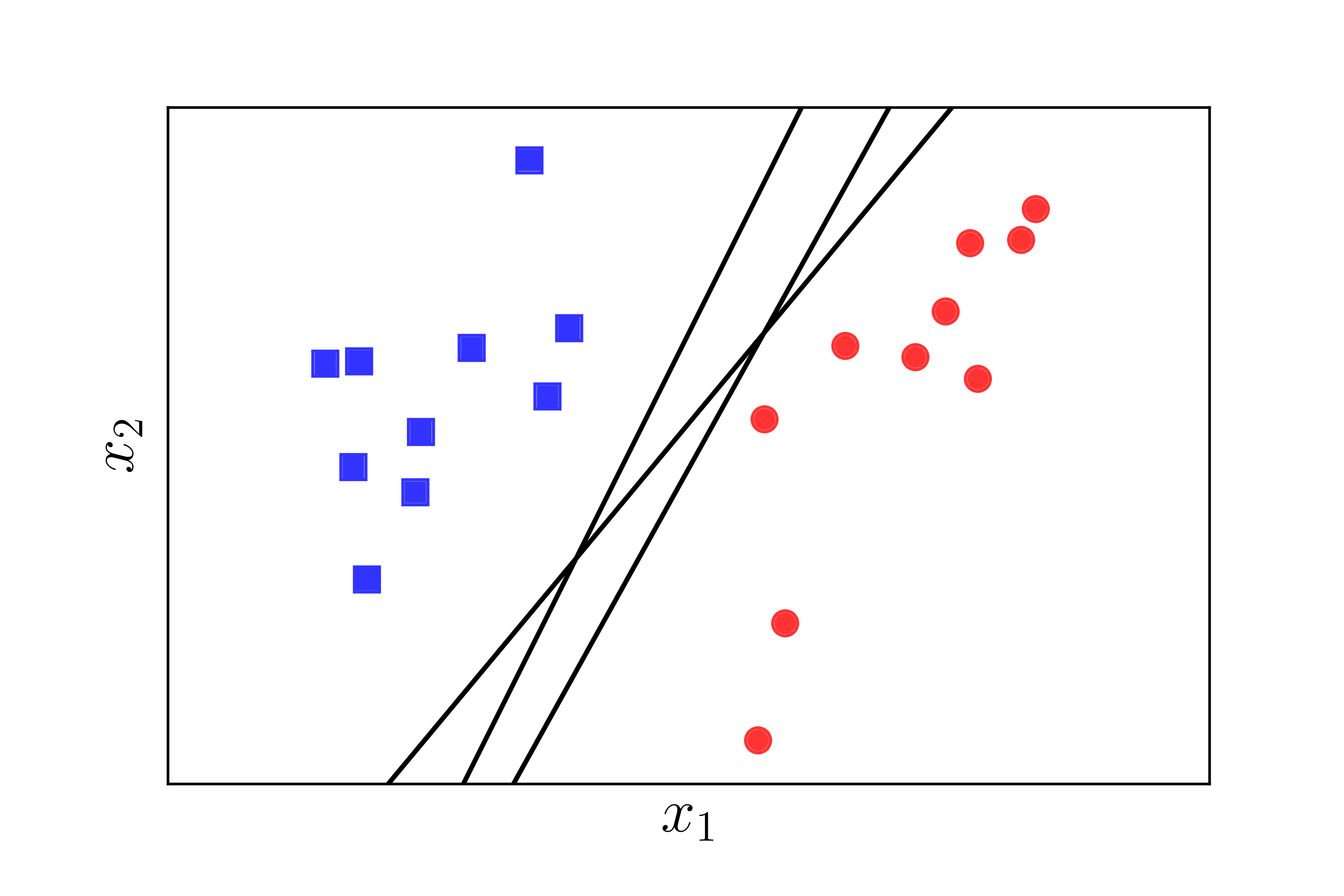
The question arises: among the many possible hyperplanes, which one is the best according to some criterion? In the three lines shown in Figure [1] above, two of them are biased towards the red circular class. This might make the red class unhappy, as it feels that its territory is being intruded upon too much. Is there a way to find a hyperplane that both classes feel is the fairest and makes them both happy?

We need a criterion to measure the happiness of each class. Let’s look at Figure 2 below:

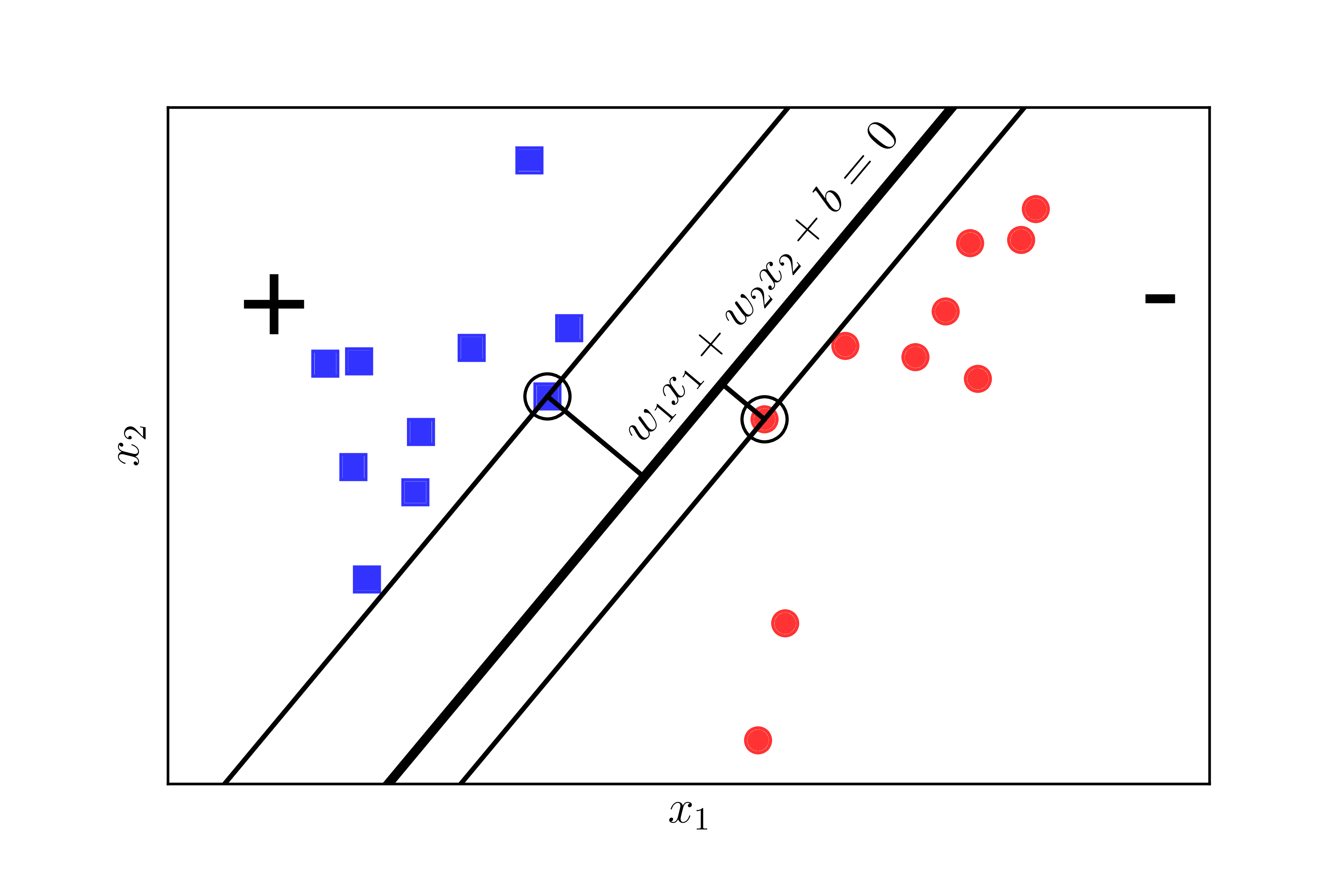
If we define the happiness of a class to be proportional to the shortest distance from a point of that class to the separating hyperplane, then in Figure [2] (left), the red circular class is not very happy because the hyperplane is much closer to it compared to the blue square class. We need a hyperplane such that the distance from the nearest point of each class (the circled points) to the hyperplane is the same, so that it is fair. This equal distance is called the margin.

Having fairness is good, but we also need equity. Fairness where both classes are equally unhappy is not quite ideal.

Now let’s consider Figure [2] (right), where the distance from the separating hyperplane to the closest points of each class is equal. Consider the two separating lines: the black solid line and the green dashed line. Which one makes both classes happier? Clearly, it is the black solid line because it creates a wider margin.

A wider margin results in better classification because the separation between the two classes is more clear-cut. This, as you will see later, is one of the key reasons why Support Vector Machine yields better classification results compared to Neural Networks with one layer, such as the Perceptron Learning Algorithm.

The optimization problem in Support Vector Machine (SVM) is to find the hyperplane such that the margin is maximized. This is why SVM is also called the Maximum Margin Classifier.

Constructing the Optimization Problem for SVM

Assume the training set consists of pairs $(\mathbf{x}_1, y_1), (\mathbf{x}_2, y_2), \dots, (\mathbf{x}_N, y_N)$, where the vector $\mathbf{x}_i \in \mathbb{R}^d$ represents the input of a data point, and $y_i$ is the label of that data point. $d$ is the number of dimensions in the data, and $N$ is the number of data points. Assume that the label of each data point is either $y_i = 1$ (class 1) or $y_i = -1$ (class 2), as in PLA.

To help visualize, consider the two-dimensional case below. The two-dimensional space is used for visualization purposes; the operations can be generalized to higher-dimensional spaces.

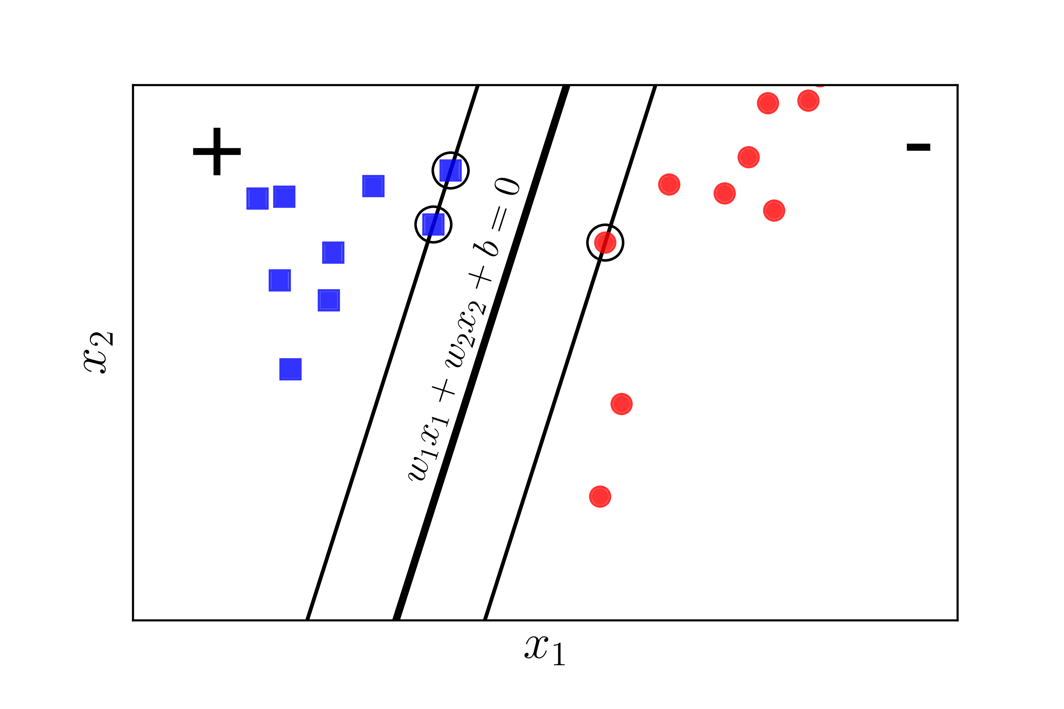
Assume that the blue square points belong to class 1, and the red circular points belong to class -1. The plane $\mathbf{w}^T\mathbf{x} + b = w_1x_1 + w_2x_2 + b = 0$ is the separating hyperplane between the two classes. Furthermore, class 1 is on the positive side, and class -1 is on the negative side of the separating plane. If the opposite were true, we would just switch the sign of $\mathbf{w}$ and $b$. Note that we need to determine the coefficients $\mathbf{w}$ and $b$.

We observe the following important point: for any data pair $(\mathbf{x}_n, y_n)$, the distance from that point to the separating plane is: $\dfrac{y_n(\mathbf{w}^T\mathbf{x}_n + b)}{|\mathbf{w}|_2}$

This is evident because, as assumed earlier, $y_n$ always has the same sign as the side of $\mathbf{x}_n$. Therefore, $y_n$ has the same sign as $(\mathbf{w}^T\mathbf{x}_n + b)$, and the numerator is always a non-negative number.

With the separating hyperplane as above, the margin is the shortest distance from any point to the plane (regardless of which point in the two classes):

The optimization problem in SVM is to find $\mathbf{w}$ and $b$ such that this margin is maximized:

Solving this problem directly is very complex, but you will see that there is a way to simplify it.

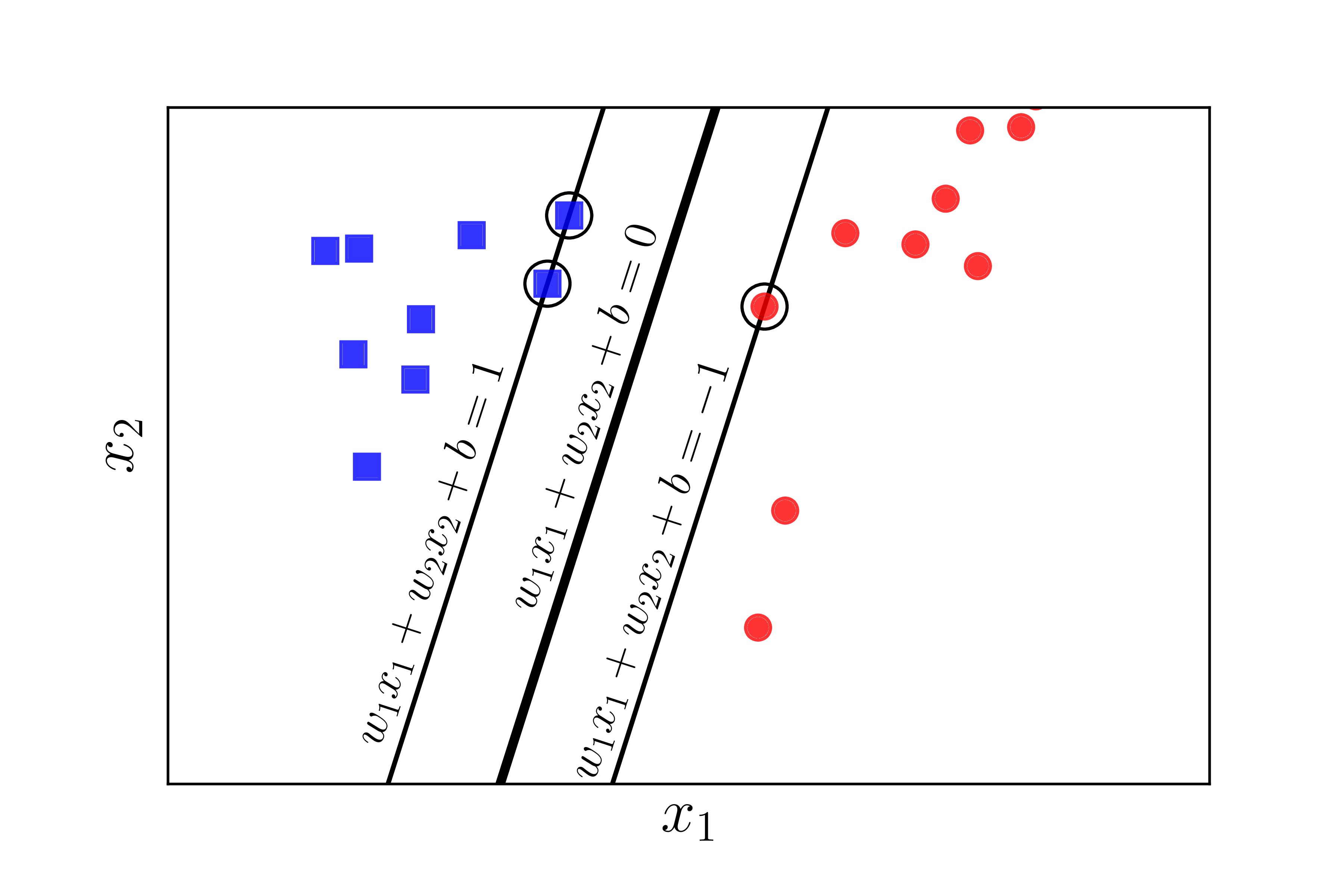
The most important observation is that if we replace the coefficient vector $\mathbf{w}$ with $k\mathbf{w}$ and $b$ with $kb$, where $k$ is a positive constant, then the separating hyperplane does not change, meaning the distance from each point to the plane remains the same, hence the margin remains unchanged. Based on this property, we can assume:

for points closest to the separating plane, as shown in Figure $\ref{fig:svm3}$ below:

Thus, for all $n$: $y_n(\mathbf{w}^T\mathbf{x}_n + b) \geq 1$

Therefore, the optimization problem $\eqref{eq:svm1}$ can be transformed into the following constrained optimization problem:

With a simple transformation, we can further reduce this to:

Here, we take the reciprocal of the objective function, square it to make it differentiable, and multiply by $\dfrac{1}{2}$ for a cleaner derivative expression.

Important Observation:

In problem $\eqref{eq:svm3}$, the objective function is a norm, which makes it convex. The inequality constraints are linear functions of $\mathbf{w}$ and $b$, so they are also convex functions. Therefore, the optimization problem $\eqref{eq:svm3}$ has a convex objective function and convex constraints, making it a convex problem. Moreover, it is a Quadratic Programming problem. The objective function is also strictly convex because $|\mathbf{w}|_2^2 = \mathbf{w}^T\mathbf{I}\mathbf{w}$, and $\mathbf{I}$ is the identity matrix—a positive definite matrix. From this, it can be concluded that the solution for SVM is unique.

At this point, this problem can be solved using tools for solving Quadratic Programming, such as CVXOPT library.

However, solving this problem becomes complicated when the dimensionality $d$ of the data space and the number of data points $N$ are large.

People often solve the dual problem of this problem. Firstly, the dual problem has interesting properties that make it more efficiently solvable. Secondly, during the formulation of the dual problem, it becomes evident that SVM can be applied to problems where the data is not linearly separable, meaning that the separating boundaries can be more complex than a simple plane.

Classifying a New Data Point: After finding the separating plane $\mathbf{w}^T\mathbf{x} + b = 0$, the class of any point is simply determined by: \(\text{class}(\mathbf{x}) = \text{sgn} (\mathbf{w}^T\mathbf{x} + b )\)

where the function $\text{sgn}$ returns 1 if the argument is non-negative and -1 otherwise.

The Dual Problem for SVM. Origin of the name "Support Vector"

Recall that the optimization problem 3 is a convex problem. We know that if a convex problem satisfies Slater’s condition, then strong duality holds. And if strong duality holds, then the solution of the problem is also the solution of the Karush-Kuhn-Tucker (KKT) conditions.

Verifying Slater’s Condition

Next, we will prove that the optimization problem 3 satisfies Slater’s condition. Slater’s condition states that if there exists $\mathbf{w}, b$ such that:

then strong duality holds.

This verification is relatively simple. Since we know that there is always a (hyper)plane that separates the two classes if they are linearly separable, meaning the problem has a solution, the feasible set of the optimization problem 3 must be non-empty. Therefore, there always exists a pair $(\mathbf{w}_0, b_0)$ such that:

Thus, simply choosing $\mathbf{w}_1 = 2\mathbf{w}_0$ and $b_1 = 2b_0$, we get:

Hence, Slater’s condition is satisfied.

Lagrangian for the SVM Problem

The Lagrangian for the optimization problem 3 is:

where $\lambda = [\lambda_1, \lambda_2, \dots, \lambda_N]^T$ and $\lambda_n \geq 0, \, \forall n = 1, 2, \dots, N$.

Lagrange Dual Function The Lagrange dual function is defined as:

where $\lambda \succeq 0$.

The minimization of this function with respect to $\mathbf{w}$ and $b$ can be carried out by solving the system of partial derivative equations of $\mathcal{L}(\mathbf{w}, b, \lambda)$ with respect to $\mathbf{w}$ and $b$, setting them to zero:

Substituting Equation 5 and Equation 6 back into Equation 4, we obtain:

This is the most important function in SVM.

Consider the matrix:

and the vector $\mathbf{1} = [1, 1, \dots, 1]^T$, we can rewrite $g(\lambda)$ as:

Define $\mathbf{K} = \mathbf{V}^T \mathbf{V}$, and we have an important observation: $\mathbf{K}$ is a positive semidefinite matrix. Indeed, for any vector $\lambda$:

The above inequation is the definition of a positive semidefinite matrix.

Thus, $g(\lambda) = -\dfrac{1}{2} \lambda^T \mathbf{K} \lambda + \mathbf{1}^T \lambda$ is a concave function.

The Lagrange Dual Problem

From here, combining the Lagrange dual function and the constraints on $\lambda$, we obtain the Lagrange dual problem:

The second constraint is derived from Equation 6. This is a convex problem because we are maximizing a concave objective function over a polyhedron. This problem is also a Quadratic Programming (QP) problem and can be solved using libraries like CVXOPT.

In this dual problem, the number of parameters to be found is $N$, which is the dimension of $\lambda$, i.e., the number of data points. Meanwhile, in the primal problem 3, the number of parameters to be found is $d + 1$, which is the total dimension of $\mathbf{w}$ and $b$, i.e., the number of dimensions of each data point plus one. In many cases, the number of data points in the training set is much greater than the number of dimensions. If solved directly using Quadratic Programming tools, the dual problem can sometimes be more complex (and take more time) than the primal problem. However, the dual problem is particularly appealing in the context of Kernel Support Vector Machine (Kernel SVM), which applies to problems where the data is not linearly separable or only nearly linearly separable. Additionally, based on the special properties of the KKT conditions, SVM can be solved using more efficient methods.

KKT Conditions

Returning to the problem, since this is a convex problem with strong duality, the solution of the problem will satisfy the KKT conditions with variables $\mathbf{w}, b$, and $\lambda$:

Among these conditions, condition $\eqref{eq:11}$ is called the complimentary slackness, and is the most interesting. From it, we can immediately deduce that for any $n$, either $\lambda_n = 0$ or $1 - y_n(\mathbf{w}^T \mathbf{x}_n + b) = 0$. The latter case corresponds to:

with the note that $y_n^2 = 1, \, \forall n$.

The points that satisfy $\eqref{eq:14}$ are the ones closest to the separating hyperplane, and they are the points circled in Figure 3{reference-type=”ref” reference=”fig:svm3”} above. The two lines $\mathbf{w}^T \mathbf{x}_n + b = \pm 1$ rest on the points that satisfy $\eqref{eq:14}$. Therefore, the points (vectors) that satisfy $\eqref{eq:14}$ are called Support Vectors. This is where the name Support Vector Machine comes from.

Another observation is that the number of points satisfying $\eqref{eq:14}$ is often very small compared to the $N$ points. Using only these support vectors, we can determine the separating hyperplane. From another perspective, most $\lambda_n$ are zero. Thus, although the vector $\lambda \in \mathbb{R}^N$ can have a large number of dimensions, the number of nonzero components is very small. In other words, the vector $\lambda$ is a sparse vector. Therefore, Support Vector Machine is also classified as a Sparse Model. Sparse Models often have more efficient (faster) solutions compared to similar models with dense solutions (most components nonzero). This is the second reason why the dual problem of SVM is often more interesting than the primal problem.

Continuing the analysis, for problems with a small number of data points $N$, the KKT conditions above can be solved by considering the cases where $\lambda_n = 0$ or $\lambda_n \neq 0$. The total number of cases to consider is $2^N$. With $N > 50$ (which is often the case), this number is very large, and solving this way becomes infeasible. I will not go deeper into how to solve the KKT system; in the next section, we will solve the optimization problem $\eqref{eq:9}$ using CVXOPT and the ‘sklearn’ library.

After finding $\lambda$ from problem $\eqref{eq:9}$, we can determine $\mathbf{w}$ using $\eqref{eq:12}$ and $b$ using $\eqref{eq:11}$ and $\eqref{eq:13}$. Clearly, we only need to consider $\lambda_n \neq 0$.

Define the set $\mathcal{S} = {n: \lambda_n \neq 0}$ and let $N_{\mathcal{S}}$ be the number of elements in the set $\mathcal{S}$. For each $n \in \mathcal{S}$:

Although from just one pair $(\mathbf{x}_n, y_n)$, we can immediately determine $b$ if $\mathbf{w}$ is known, another version used for computing $b$, which is often more numerically stable, is

which is the average over all calculations of $b$.

Previously, according to $\eqref{eq:12}$, $\mathbf{w}$ was computed by

Important observation: To determine which class a new point $\mathbf{x}$ belongs to, we need to determine the sign of the following expression:

This expression depends on computing the dot product between the vectors $\mathbf{x}$ and each $\mathbf{x}_n \in \mathcal{S}$. This important observation will be useful in the Kernel SVM.

SVM in Python

Solve by formula

First, we import the necessary modules and create some synthetic data (this is the same data that I used in the figures above, so we know for sure that the two classes are linearly separable):

from __future__ import print_function
import numpy as np 
import matplotlib.pyplot as plt
from scipy.spatial.distance import cdist
np.random.seed(42)

means = [[2, 2], [4, 2]]
cov = [[.3, .2], [.2, .3]]
N = 10
X0 = np.random.multivariate_normal(means[0], cov, N) # class 1
X1 = np.random.multivariate_normal(means[1], cov, N) # class -1 
X = np.concatenate((X0.T, X1.T), axis = 1) # all data 
y = np.concatenate((np.ones((1, N)), -1*np.ones((1, N))), axis = 1) # labels 

Next, we solve the problem [eq:9]{reference-type=”eqref” reference=”eq:9”} using CVXOPT:

from cvxopt import matrix, solvers
# build K
V = np.concatenate((X0.T, -X1.T), axis = 1)
K = matrix(V.T.dot(V)) # see definition of V, K near eq (8)

p = matrix(-np.ones((2*N, 1))) # all-one vector 
# build A, b, G, h 
G = matrix(-np.eye(2*N)) # for all lambda_n >= 0
h = matrix(np.zeros((2*N, 1)))
A = matrix(y) # the equality constraint is actually y^T lambda = 0
b = matrix(np.zeros((1, 1))) 
solvers.options['show_progress'] = False
sol = solvers.qp(K, p, G, h, A, b)

l = np.array(sol['x'])
print('lambda = ')
print(l.T)

The result:

    lambda = 
     [[  8.54018321e-01   2.89132533e-10   1.37095535e+00   6.36030818e-10
        4.04317408e-10   8.82390106e-10   6.35001881e-10   5.49567576e-10
        8.33359230e-10   1.20982928e-10   6.86678649e-10   1.25039745e-10
        2.22497367e+00   4.05417905e-09   1.26763684e-10   1.99008949e-10
        2.13742578e-10   1.51537487e-10   3.75329509e-10   3.56161975e-10]]

We notice that most of the values of $\lambda$ are very small, on the order of $10^{-9}$ or $10^{-10}$. These are effectively zero due to computational inaccuracies. Only three values are non-zero, so we predict that there are three support vectors.

We now find the support set $\mathcal{S}$ and solve the problem:

epsilon = 1e-6 # just a small number, greater than 1e-9
S = np.where(l > epsilon)[0]

VS = V[:, S]
XS = X[:, S]
yS = y[:, S]
lS = l[S]
# calculate w and b
w = VS.dot(lS)
b = np.mean(yS.T - w.T.dot(XS))

print('w = ', w.T)
print('b = ', b)

The result:

    w =  [[-2.00984381  0.64068336]]
    b =  4.66856063387

We illustrate the result:

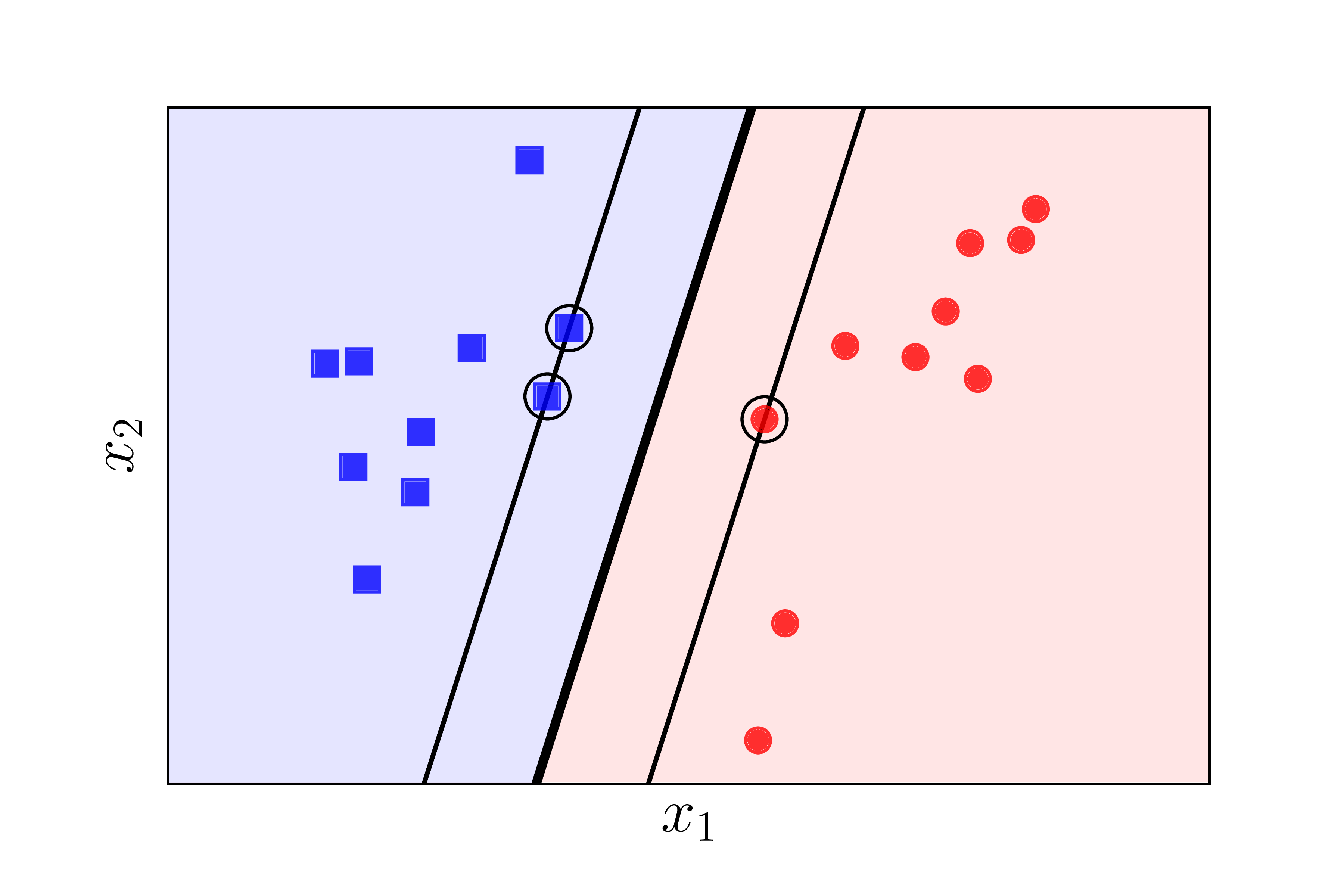
The thick black line in the middle is the separating hyperplane found by SVM. It suggests that the calculations are most likely correct. To verify, we can also solve the problem using a standard library, such as sklearn.

SVM by sklearn.svm library

We will now use the sklearn.svm.SVC built-in function.

from sklearn.svm import SVC

y1 = y.reshape((2*N,))
X1 = X.T # each sample is one row
clf = SVC(kernel = 'linear', C = 1e5) # just a big number 

clf.fit(X1, y1) 

w = clf.coef_
b = clf.intercept_
print('w = ', w)
print('b = ', b)

The result:

    w =  [[-2.00971102  0.64194082]]
    b =  [ 4.66595309]

Summary and Discussion

• For a binary classification problem where the two classes are linearly separable, there are infinitely many hyperplanes that can separate the classes. Each hyperplane defines a different classifier, and the distance from the closest point to the hyperplane is called the margin.

• The SVM problem seeks the hyperplane that maximizes the margin, ensuring that the data points are as far as possible from the separating hyperplane.

• The optimization problem in SVM is a convex problem with a strictly convex objective function, meaning the solution is unique. Additionally, the optimization problem is a Quadratic Programming (QP) problem.

• While we could directly solven the original SVM problem, it is typically solved using the dual problem, which is also a QP. The solution is sparse, making the dual problem more efficient to solve.

• For problems where the two classes are not linearly separable, we need to make sacrifices, or build another nonlinear kernel if the dataset has some special distributions (will elaborate afterwards). For n-ary classification problem, we need a Multiclass SVM (will not be elaborated as it is out-of-scope).