Soft Margin SVM

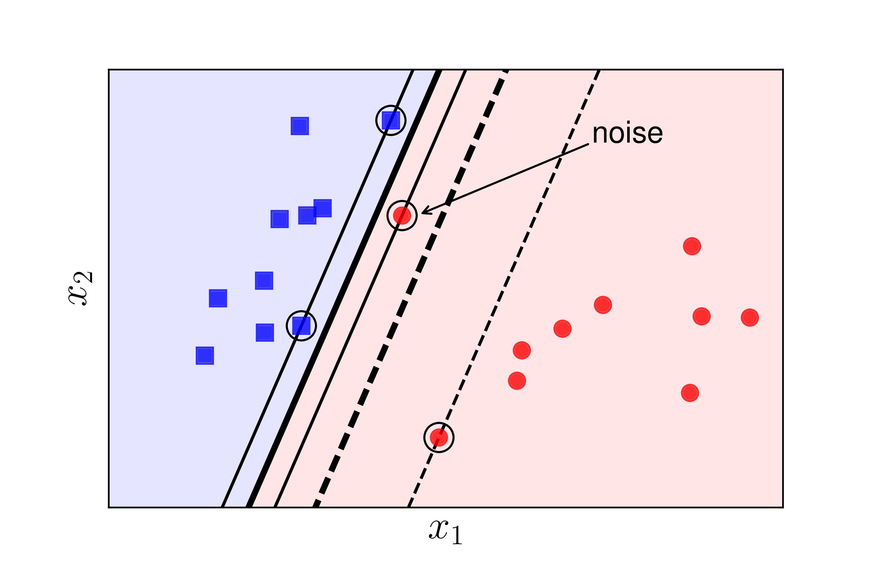
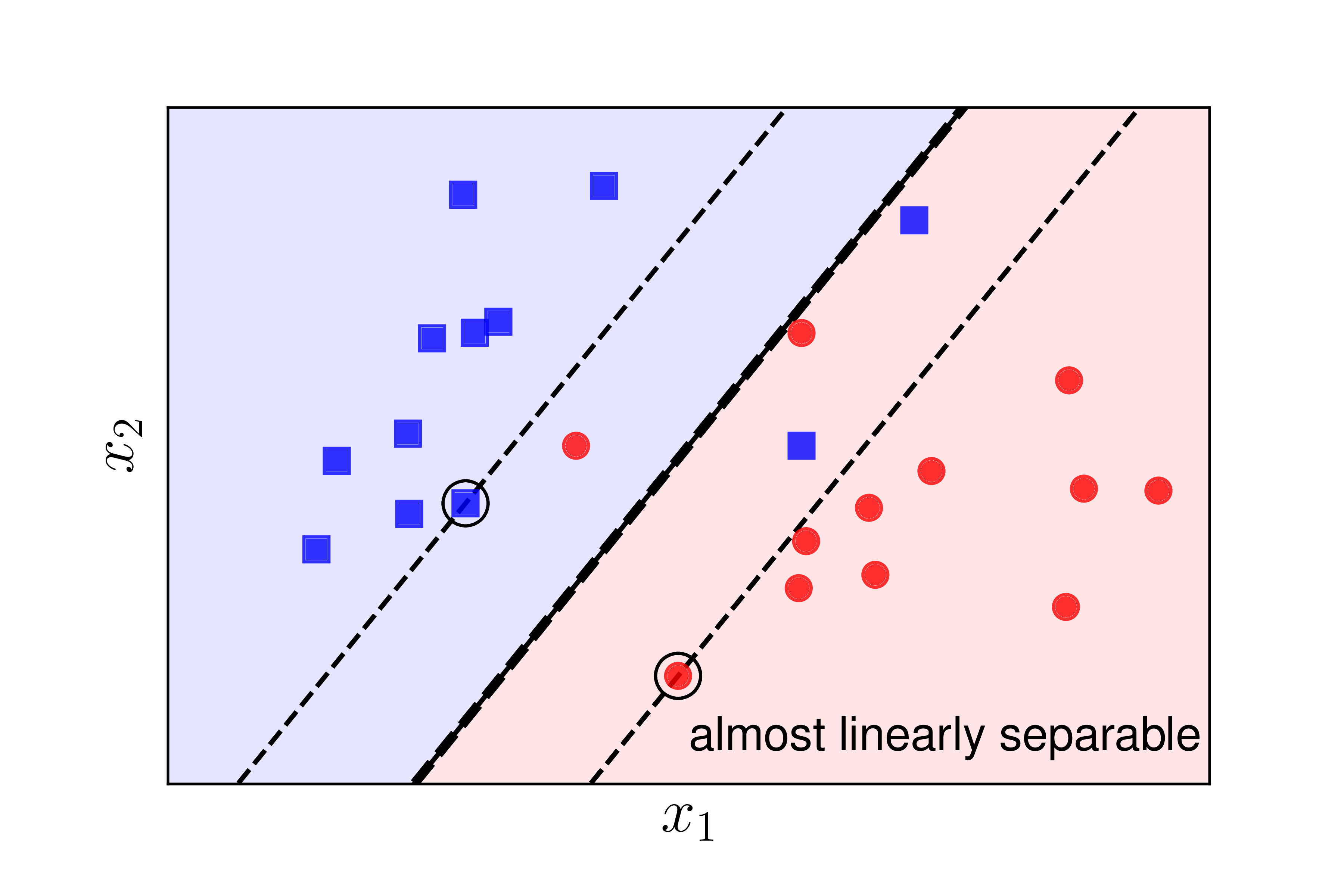
Consider two examples in Figure [2] below:

The default SVM will not work well (or even malfunction) in both cases:

• Case 1: The data is still linearly separable, but there is noise from the red circle class too close to the green square class. In this case, if we use the default SVM, it will create a very small margin. Moreover, the decision boundary will be too close to the green squares and far from the red circles. However, if we sacrifice this noise point, we can get a much better margin as illustrated by the dashed lines. Therefore, the default SVM is also considered noise sensitive.

• Case 2: The data is not linearly separable but is nearly linearly separable like in Figure [2]. In this case, if we use the default SVM, the optimization problem becomes infeasible, meaning the feasible set is empty, and the SVM optimization problem has no solution. However, if we sacrifice a few points near the boundary between the two classes, we can still create a good decision boundary, like the thick dashed line. The support lines formed by thin dashed lines still help create a large margin for this classifier. Each point that crosses over to the other side of the support lines (or margin lines or boundary lines) is considered to fall into the unsafe region. Note that the safe regions of the two classes are different, and they overlap in the area between the two support lines.

In both cases, the margin created by the decision boundary and the thin dashed lines is referred to as a soft margin. Similarly, the default SVM is also known as a Hard Margin SVM.

In this section, we will explore a variant of the Hard Margin SVM known as the Soft Margin SVM.

The optimization problem for the Soft Margin SVM can be approached in two different ways, both of which yield interesting results and can be extended into more complex and effective SVM algorithms.

The first approach is to solve a constrained optimization problem by solving the dual problem, similar to the Hard Margin SVM. The dual approach lays the foundation for the Kernel SVM for data that is truly not linearly separable.

The second approach is to turn the problem into an unconstrained optimization problem. This problem can be solved using Gradient Descent methods. Therefore, this approach can be applied to large-scale problems. Additionally, in this solution, we will introduce a new loss function called the hinge loss. This loss function can be extended to the multi-class classification problem, which will be elaborate further on in the section of Multiclass SVM.

Let’s first analyze the problem.

Mathematical Analysis

As mentioned above, to achieve a larger margin in Soft Margin SVM, we need to sacrifice some data points by allowing them to fall into the unsafe region. Of course, we must limit this sacrifice; otherwise, we could create a very large margin by sacrificing most points. Therefore, the objective function should be a combination that maximizes the margin and minimizes the sacrifice.

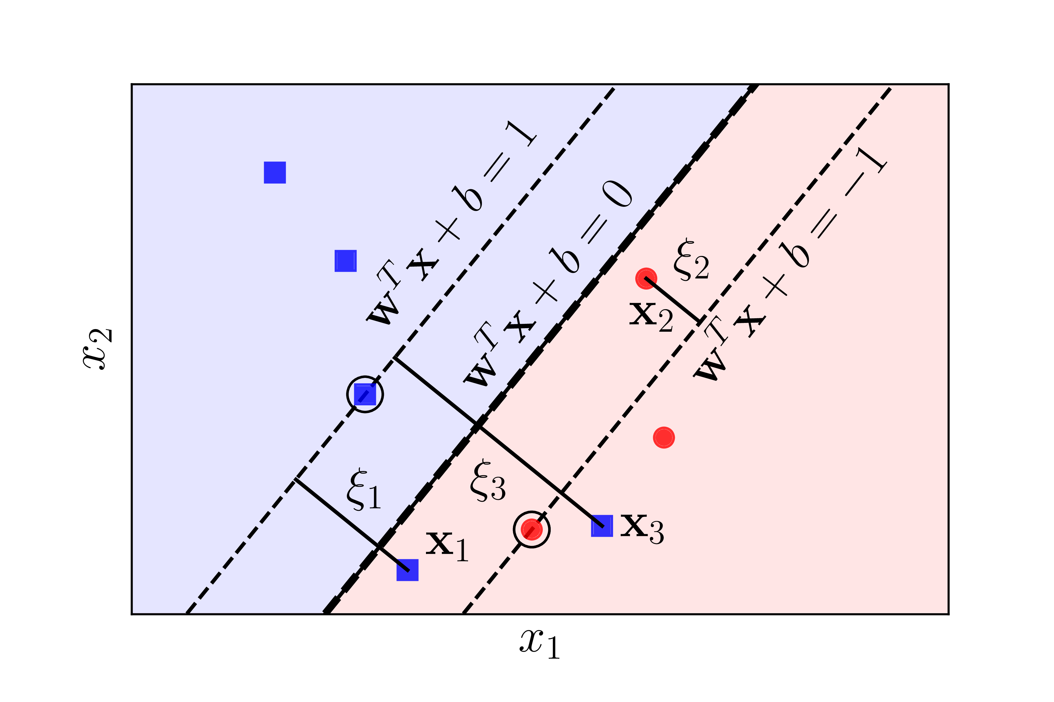
Like in the Hard Margin SVM, maximizing the margin can be reduced to minimizing $|\mathbf{w}|_2^2$. To define the sacrifice, let’s refer to Figure [3] below:

Introducing slack variables $\xi_n$. For points within the safe region, $\xi_n = 0$. Points in the unsafe region but still on the correct side of the boundary correspond to $0 < \xi_n < 1$, for example, $\mathbf{x}_2$. Points on the wrong side of the boundary for their class correspond to $\xi_n > 1$, for example, $\mathbf{x}_1$ and $\mathbf{x}_3$.

For each point $\mathbf{x}_n$ in the entire training dataset, we introduce a slack variable $\xi_n$ that measures the sacrifice. This variable is also known as the slack variable. For points $\mathbf{x}_n$ within the safe region, $\xi_n = 0$. For points in the unsafe region like $\mathbf{x}_1$, $\mathbf{x}_2$, or $\mathbf{x}_3$, we have $\xi_n > 0$.

If $y_i= \pm 1$ is the label of $\mathbf{x}_i$ in the unsafe region, then $\xi_i = |\mathbf{w}^T\mathbf{x}_i + b - y_i|$.

Let’s recall the optimization problem for the Hard Margin SVM:

\[\begin{aligned} (\mathbf{w}, b) &=& \arg \min_{\mathbf{w}, b} \dfrac{1}{2} \|\mathbf{w}\|_2^2 \\ \text{subject to:}&& \, y_n(\mathbf{w}^T \mathbf{x}_n + b) \geq 1, \, \forall n = 1, 2, \dots, N \end{aligned}\]

For the Soft Margin SVM, the objective function will include an additional term to minimize the sacrifice. Therefore, the objective function becomes:

\[\dfrac{1}{2} \|\mathbf{w}\|_2^2 + C \sum_{n=1}^N \xi_n\]

where $C$ is a positive constant, and $\xi = [\xi_1, \xi_2, \dots, \xi_N]$.

The constant $C$ is used to adjust the balance between the margin and the sacrifice. This constant is pre-determined by the programmer or can be set via cross-validation.

The constraints will change slightly. For each data pair $(\mathbf{x}_n, y_n)$, instead of a hard constraint $y_n(\mathbf{w}^T \mathbf{x}_n + b) \geq 1$, we will have a soft constraint:

\[\begin{aligned} && y_n(\mathbf{w}^T \mathbf{x}_n + b) \geq 1 - \xi_n, \forall n = 1, 2, \dots, N \nonumber \\ &\Leftrightarrow& 1 - \xi_n - y_n(\mathbf{w}^T \mathbf{x}_n + b) \leq 0, \, \forall n = 1, 2, \dots, N \nonumber \end{aligned}\]

And an additional constraint: $\xi_n \geq 0, \forall n = 1, 2, \dots, N$.

In summary, we have the optimization problem in standard form for Soft-margin SVM:

\[\begin{aligned} (\mathbf{w}, b, \xi) &=& \arg \min_{\mathbf{w}, b, \xi} \dfrac{1}{2} \|\mathbf{w}\|_2^2 + C \sum_{n=1}^N \xi_n \nonumber \\ \text{subject to:}&& \, 1 - \xi_n - y_n(\mathbf{w}^T \mathbf{x}_n + b) \leq 0, \forall n = 1, 2, \dots, N \label{eq:soft2}\\ && - \xi_n \leq 0, \, \forall n = 1, 2, \dots, N \nonumber \end{aligned}\]

Notes:

• When $C$ is small, the sacrification does not have much effect on the objective function. The algorithm will automatically adapt and minimize \(\|\|\mathbf{x}\|\|_2^2\), or maximize margin, further increasing the sum \(\sum_{n=1}^N\xi_n\).

• The optimization problem 2 has slack variables $\xi_n$. Data points with $\xi_n = 0$ are in the safe region (satisfy constraint $y_n(\mathbf{w}^T \mathbf{x}_n + b) \geq 1$), while data points with $0 < \xi_n \leq 1$ are in the unsafe region (correctly classified but are too close to the hyperplane), and data points with $\xi_n > 1$ are misclassified.

• The objective function is convex as it is the sum of two convex functions: the norm function and the linear function. The constraints are also convex. Therefore, this is a convex optimization problem, meaning that the local optimum is the global optimum.

Below, we will solve the optimization problem 2 in two different ways.

Lagrange Dual Problem

Note that this problem can be directly solved using QP toolboxes, but similar to the Hard Margin SVM, we will focus more on the dual problem.

First, we need to check the Slater’s condition for the convex optimization problem 2. If this condition is satisfied, then strong duality will also hold, meaning the solution of the optimization problem 2 is the same as the solution of the KKT conditions.

Checking Slater’s Condition

It is clear that for all $n = 1, 2, \dots, N$ and for all $(\mathbf{w}, b)$, we can always find positive values of $\xi_n, n = 1, 2, \dots, N$ that are large enough so that:

$y_n(\mathbf{w}^T\mathbf{x}_n + b) + \xi_n > 1, \quad \forall n = 1, 2, \dots, N$

Therefore, this problem satisfies Slater’s condition.

Lagrangian of the Soft-margin SVM Problem

The Lagrangian for problem $\eqref{eq:soft2}$ is:

\[\mathcal{L}(\mathbf{w}, b, \xi, \lambda, \mu) = \dfrac{1}{2} \|\mathbf{w}\|_2^2 + C \sum_{n=1}^N \xi_n + \sum_{n=1}^N \lambda_n (1 - \xi_n - y_n(\mathbf{w}^T\mathbf{x}_n + b)) - \sum_{n=1}^N \mu_n \xi_n \label{eq:soft3}\]

where $\lambda = [\lambda_1, \lambda_2, \dots, \lambda_N]^T \succeq 0$ and $\mu = [\mu_1, \mu_2, \dots, \mu_N]^T \succeq 0$ are the Lagrange dual variables.

Dual Problem

The dual function for the optimization problem $\eqref{eq:soft2}$ is:

\[g(\lambda, \mu) = \min_{\mathbf{w}, b, \xi} \mathcal{L}(\mathbf{w}, b, \xi, \lambda, \mu)\]

For each pair $(\lambda, \mu)$, we consider $(\mathbf{w}, b, \xi)$ that satisfies the condition that the derivative of the Lagrangian is equal to 0:

\[\begin{aligned} \dfrac{\partial \mathcal{L}}{\partial \mathbf{w}} & =& 0 \quad \Leftrightarrow \quad \mathbf{w} = \sum_{n=1}^N \lambda_n y_n \mathbf{x}_n \label{eq:4_constraints} \\ \dfrac{\partial \mathcal{L}}{\partial b} & =& 0 \quad \Leftrightarrow \quad \sum_{n=1}^N \lambda_n y_n = 0 \label{eq:5_constraints} \\ \dfrac{\partial \mathcal{L}}{\partial \xi_n} & =& 0 \quad \Leftrightarrow \quad \lambda_n = C - \mu_n \label{eq:6_constraints} \end{aligned}\]

From $\eqref{eq:6_constraints}$, we can see that we only consider pairs $(\lambda, \mu)$ such that $\lambda_n = C - \mu_n$. From here, we also have $0 \leq \lambda_n, \mu_n \leq C, \, n = 1, 2, \dots, N$. Substituting these expressions into the Lagrangian, we get the dual function:

\[g(\lambda, \mu) = \sum_{n=1}^N \lambda_n - \dfrac{1}{2} \sum_{n=1}^N \sum_{m=1}^N \lambda_n \lambda_m y_n y_m \mathbf{x}_n^T \mathbf{x}_m\]

Note that this function does not depend on $\mu$, but we need to consider the constraint $~\eqref{eq:6_constraints}$. This constraint, along with the non-negativity condition on $\lambda$, can be rewritten as $0 \leq \lambda_n \leq C$, effectively reducing the variable $\mu$. Now, the dual problem is given by:

\[\begin{aligned} \lambda &=& \arg \max_{\lambda} g(\lambda) \nonumber \\ \text{subject to:} && \sum_{n=1}^N \lambda_n y_n = 0, \label{eq:7_constraints} \\ && 0 \leq \lambda_n \leq C, \, \forall n = 1, 2, \dots, N \label{eq:8_constraints} \end{aligned}\]

This problem is similar to the [dual problem of the Hard Margin SVM, except that there is an upper bound on each $\lambda_n$. When $C$ is very large, the two problems can be considered the same. The constraint $~\eqref{eq:8_constraints}$ is also known as a box constraint because the feasible set of points $\lambda$ satisfying this constraint forms a rectangular box in high-dimensional space.

This problem can also be solved entirely using standard QP solvers such as CVXOPT, as I did in the Hard Margin SVM example.

After finding $\lambda$ from the dual problem, we still need to find the solution $(\mathbf{w}, b, \xi)$ of the original problem. To do this, we need to examine the KKT conditions.

KKT Conditions

The KKT conditions for the optimization problem of Soft Margin SVM are, for all $n = 1, 2, \dots, N$:

\[\begin{aligned} 1 - \xi_n - y_n(\mathbf{w}^T\mathbf{x}_n + b) &\leq& 0 \\ -\xi_n &\leq& 0 \\ \lambda_n &\geq& 0 \\ \mu_n &\geq& 0 \label{eq:soft12} \\ \lambda_n (1 - \xi_n - y_n(\mathbf{w}^T\mathbf{x}_n + b)) &=& 0 \label{eq:soft13} \\ \mu_n \xi_n &=& 0 \label{eq:soft14} \\ \mathbf{w} &=& \sum_{n=1}^N \lambda_n y_n \mathbf{x}_n \nonumber \\ \sum_{n=1}^N \lambda_n y_n &=& 0 \nonumber \\ \lambda_n &=& C - \mu_n \nonumber \end{aligned}\]

(To make it easier to visualize, I have rewritten conditions $~\eqref{eq:4_constraints}, ~\eqref{eq:5_constraints}, ~\eqref{eq:6_constraints}$ in this system.)

We can make some observations:

• If $\lambda_n = 0$, then from $\eqref{eq:6_constraints}$, we have $\mu_n = C \neq 0$. Combining this with $\eqref{eq:soft14}$, we get $\xi_n = 0$. In other words, no sacrifice occurs at $\mathbf{x}_n$, meaning $\mathbf{x}_n$ lies in the safe region.

• If $\lambda_n > 0$, from $\eqref{eq:soft13}$, we have: $y_n(\mathbf{w}^T \mathbf{x}_n + b) = 1 - \xi_n$

• If $0 < \lambda_n < C$, from $~\eqref{eq:6_constraints}$, we have $\mu_n \neq 0$, and from $(14)$, we have $\xi_n = 0$. In other words, $y_n(\mathbf{w}^T \mathbf{x}_n + b) = 1$, meaning these points lie exactly on the margin.

• If $\lambda_n = C$, then $\mu_n = 0$, and $\xi_n$ can take any non-negative value. If $\xi_n \leq 1$, $\mathbf{x}_n$ will be correctly classified (still on the correct side of the decision boundary). Otherwise, for points with $\xi_n > 1$, they will be misclassified.

• $\lambda_n$ cannot be greater than $C$ because then, according to $\eqref{eq:6_constraints}$, $\mu_n < 0$, which contradicts $\eqref{eq:soft12}$.

In addition, the points corresponding to $0 < \lambda_n \leq C$ are now considered support vectors. Although these points may not lie on the margins, they are still considered support vectors because they contribute to the computation of $\mathbf{w}$ through equation $(4)$.

Thus, based on the values of $\lambda_n$, we can predict the relative position of $\mathbf{x}_n$ with respect to the two margins. Define $\mathcal{M} = {n: 0 < \lambda_n < C}$ and $\mathcal{S} = {m: 0 < \lambda_m \leq C}$. That is, $\mathcal{M}$ is the set of indices of points that lie exactly on the margins—used to calculate $b$, and $\mathcal{S}$ is the set of indices of the support vectors—used directly to calculate $\mathbf{w}$. Similar to the Hard Margin SVM, the parameters $\mathbf{w}, b$ can be determined by:

\[\begin{aligned} \mathbf{w} &=& \sum_{m \in \mathcal{S}} \lambda_m y_m \mathbf{x}_m \label{eq:soft15} \\ b &=& \dfrac{1}{N_{\mathcal{M}}} \sum_{n \in \mathcal{M}} \left( y_n - \mathbf{w}^T \mathbf{x}_n \right) = \dfrac{1}{N_{\mathcal{M}}} \sum_{n \in \mathcal{M}} \left( y_n - \sum_{m \in \mathcal{S}} \lambda_m y_m \mathbf{x}_m^T \mathbf{x}_n \right) \label{eq:soft16} \end{aligned}\]

Note that the ultimate goal is to determine the label for a new point, not to compute $\mathbf{w}$ and $b$, so we are more interested in determining the value of the following expression for any data point $\mathbf{x}$:

\[\mathbf{w}^T \mathbf{x} + b = \sum_{m \in \mathcal{S}} \lambda_m y_m \mathbf{x}_m^T \mathbf{x} + \dfrac{1}{N_{\mathcal{M}}} \sum_{n \in \mathcal{M}} \left( y_n - \sum_{m \in \mathcal{S}} \lambda_m y_m \mathbf{x}_m^T \mathbf{x}_n \right)\]

In this calculation, we only need to consider the inner product between any two points.