Classification model

Logistic Regression

Symbol	Definition
$x$	training example feature values
$y$	training example targets
$w$	weight parameter
$b$	bias parameter
$m$	number of training examples in the data set
$n$	number of features
$i$	the $i^{th}$ training example in the data set
$j$	the $j^{th}$ feature
$x_j^{(i)}$	value of the $j^{th}$ feature in the $i^{th}$ training example
$w_j^{(i)}$	weight of the $j^{th}$ feature
$f_{\vec{w},b}(\vec{x}^{(i)})$	model’s result of the $i^{th}$ training example
$\hat{y}^{(i)}$	model’s prediction of the $i^{th}$ training example
$y^{(i)}$	target of the $i^{th}$ training example
$z$	decision boundary
$g(\vec{w}.\vec{x} + b)$	logistic function
$L(f_{\vec{w},b}(\vec{x}^{(i)}), y^{(i)})$	loss function
$J(\vec{w},b)$	cost function
$\alpha$	learning rate

Logistic function

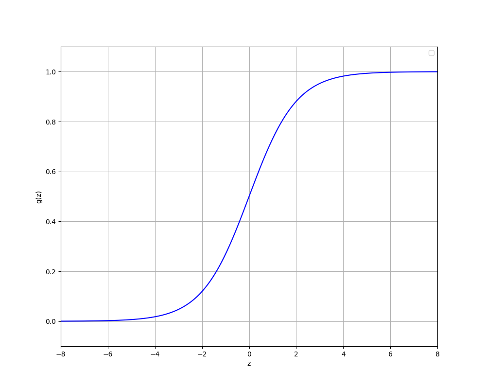
Logistic function is one of sigmoid functions which is commonly applied in logistic regression. We want prediction $\hat{y}$ between 0 and 1 then logistic functions are appropriate to apply.

\[g(z) = \frac{1}{1+e^{-z}} \text{ ($0 < g(z) < 1$)}\] \[z = \vec{w}.\vec{x} + b\] \[f_{\vec{w},b}(\vec{x}) = g(\vec{w}.\vec{x} + b) = \frac{1}{1+e^{-(\vec{w}.\vec{x} + b)}}\]

Decision boundary

\[P(y=1|x; \vec{w},b) \text{ or } \hat{y} = 1\] \[\text{when }f_{\vec{w},b}(\vec{x}) \geq 0.5 \text{ (threshold)}\] \[g(z) \geq 0.5\] \[z \geq 0\]

In this case, we say that decision boundary is z = 0.

$z \geq 0$	$z < 0$
$\vec{w}.\vec{x} + b \geq 0$	$\vec{w}.\vec{x} + b < 0$
$\hat{y} = 1$	$\hat{y} = 0$

Note: Threshold no need to be 0.5. For example, tumor positive(1) malignant, negative(0) be nign, we tend to get a low threshold such as 0.2 or 0.1 for a tumor detection algorithm because we would not like to miss a potential tumor. In contrast, in our project AI-generated text detector with positive(1) AI-generated and negative(0) human-written, we tend to get a high threshold as the consequence of accusing someone of cheating with AI-generated text is more severe than missing. Then, decision boundary = z = $-\log(\frac{1}{\mathbf{threshold}} - 1)$

Cross-Entropy Loss function

Loss $L(f_{\vec{w},b}(\vec{x}^{(i)}), y^{(i)})$ is a measure of the difference of a single example to its target value.
if $y^{(i)} = 1:$ We want a loss function that when $f_{\vec{w},b}(\vec{x}^{(i)})$ reach 1, the loss reach 0 and when $f_{\vec{w},b}(\vec{x}^{(i)})$ reach 0, the loss become higher. Then, $-\log(f_{\vec{w},b}(\vec{x}^{(i)}))$ is suitable.

\[L(f_{\vec{w},b}(\vec{x}^{(i)}), y^{(i)}) = -\log(f_{\vec{w},b}(\vec{x}^{(i)}))\]

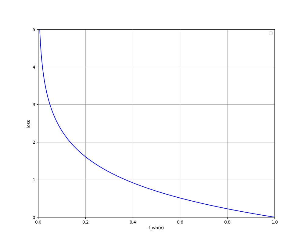
if $y^{(i)} = 0:$ We want a loss function that when $f_{\vec{w},b}(\vec{x}^{(i)})$ reach 0, the loss reach 0 and when $f_{\vec{w},b}(\vec{x}^{(i)})$ reach 1, the loss become higher. Then, $-log(1-f_{\vec{w},b}(\vec{x}^{(i)}))$ is suitable.

\[L(f_{\vec{w},b}(\vec{x}^{(i)}), y^{(i)}) = -\log(1 - f_{\vec{w},b}(\vec{x}^{(i)}))\]

We have:

\[L(f_{\vec{w},b}(\vec{x}^{(i)}), y^{(i)}) = \begin{cases} -\log(f_{\vec{w},b}(\vec{x}^{(i)}))& \text{if $y^{(i)} = 1$} \\ -\log(1 - f_{\vec{w},b}(\vec{x}^{(i)})) & \text{if $y^{(i)} = 0$} \end{cases}\]

Therefore:

\[L(f_{\vec{w},b}(\vec{x}^{(i)}), y^{(i)}) = -y^{(i)}\log(f_{\vec{w},b}(\vec{x}^{(i)})) - (1-y^{(i)})\log(1 - f_{\vec{w},b}(\vec{x}^{(i)}))\]

Cost function

Cost $J(\vec{w},b)$ is a measure of the losses over the training set

\[J(\vec{w},b) = \frac{1}{m}\sum_{i=0}^{m-1}[{L(f_{\vec{w},b}(\vec{x}^{(i)}), y^{(i)})]}\]

Our objective is to minimise the cost function and this problem can be reasonably solved by applying gradient descent.

Gradient descent

Gradient descent is a good way to help us reduce the cost of the model by picking the weight and bias parameters that give the smallest possible value of $J(\vec{w},b)$. In detail, we will start with some w and b, for instance, we can set $\vec{w} = \vec{0}$ and b = 0. After that, we keep changing w, b to reduce $J(\vec{w},b)$ until we level off at the minimum of cost $J(\vec{w},b)$. Let get parameter $w_j$ as an example, the partial derivatives $\frac{\partial J({w},b)}{\partial w_j}$at a point on the cost function $J(\vec{w},b)$ curve is illustrated as slope of the tangent line at that point.

Case 1: when the optimization point of $w_j$ for minimum the cost $J(\vec{w},b)$ is less than the current $w_j$, we want to move $w_j$ to the left, so $w_j$ should minus a positive number to end up with a new smaller value $w_j$.

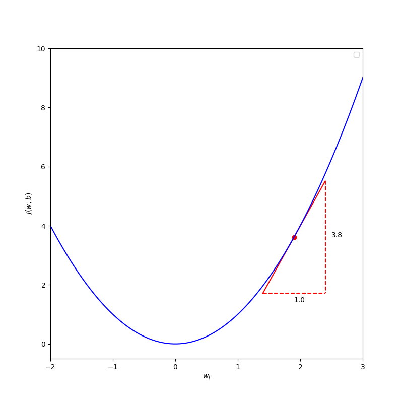
We have learning rate $\alpha$ is a positive number and the tangent line is pointing up to the right that lead the slope to be positive, which means that the derivative $\frac{\partial J({w},b)}{\partial w_j}$ is a positive number.

\[w_j = w_j - \alpha \frac{\partial J(\vec{w},b)}{\partial w_j}\] \[w_j = w_j - \text{(positive number)} * \text{(positive number)}\] \[w_j = w_j - \text{(positive number)}\] \[\text{then }w_j \text{ will become smaller}\] \[\text{thus, }w_j \text{ move to the left}\]

Case 2: when the optimization point of $w_j$ for minimum the cost $J(\vec{w},b)$ is greater than the current $w_j$, we want to move $w_j$ to the right, so $w_j$ should minus a negative number to end up with a new larger value $w_j$.

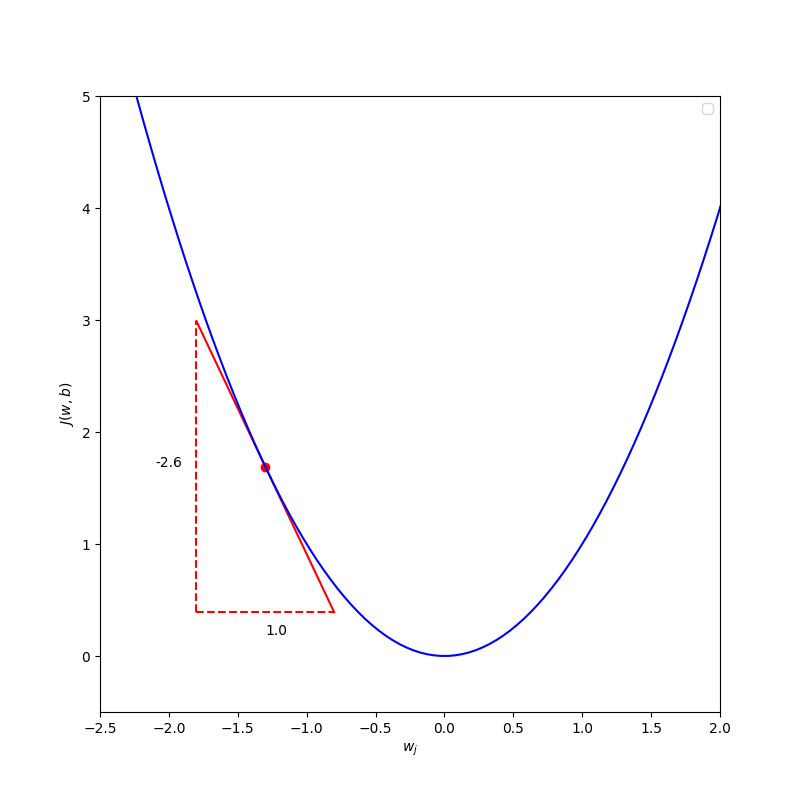
We have learning rate $\alpha$ is a positive number and the tangent line is pointing down to the right that lead the slope to be negative, which means that the derivative $\frac{\partial J({w},b)}{\partial w_j}$ is a negative number. \(w_j = w_j - \alpha \frac{\partial J(\vec{w},b)}{\partial w_j}\) \(w_j = w_j - \text{(positive number)} * \text{(negative number)}\) \(w_j = w_j - \text{(negative number)}\) \(\text{then }w_j \text{ will become larger}\) \(\text{thus, }w_j \text{ move to the right}\)

In both cases, we take the same function $w_j = w_j - \alpha \frac{\partial J({w},b)}{\partial w_j}$. Therefore, we will change simultaneously all parameters w and b by applying the same method that the parameters are updated to be minus the learning rate times the derivative term.

\[\begin{aligned} &\\ & \frac{\partial J(\vec{w},b)}{\partial w_j} = \frac{1}{m} \sum\limits_{i = 0}^{m-1} (f_{\vec{w},b}(\vec{x}^{(i)}) - y^{(i)})x_{j}^{(i)} \\ & \frac{\partial J(\vec{w},b)}{\partial b} = \frac{1}{m} \sum\limits_{i = 0}^{m-1} (f_{\vec{w},b}(\vec{x}^{(i)}) - y^{(i)}) \\ & w_j = w_j - \alpha \frac{\partial J(\vec{w},b)}{\partial w_j} \; & \text{for j := 0..n-1} \\ & b = b - \alpha \frac{\partial J(\vec{w},b)}{\partial b} \\ & \end{aligned}\]

Nevertheless, the gradient descent can make the cost $J(\vec{w},b)$ stuck at a local minimum, which not the global minimum so that we should differentiate the starting point of parameters $\vec{w}$ and b. Let get $J(w)$ as an example:

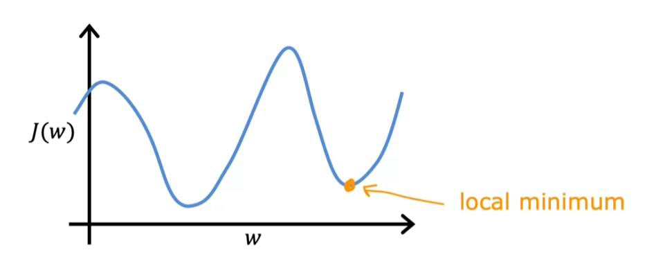
Learning rate

As choosing a learning rate affects intensively the efficiency when implementing gradient descent, we will go through this concept. The learning rate $\alpha$ is a tuning positive number that settles the variation of the parameters w and b at each iteration while the cost function $J(\vec{w},b)$ approaches the minimum.If $\alpha$ is too small, the gradient descent may slowly move the cost toward the minimum and the program break before the cost reach end up at the local minimum. However, a large $\alpha$ can lead the the cost to overshoot and never reach minimum. We ordinarily set $\alpha = 10^{-3}$, although we should manipulate the learning rate so as to get the appropriate value for the learning model. With an easy approach, we can set $\alpha = 1$ as a high learning at the beginning, if the cost is divergent, we moderate $\alpha$ by reducing it by 3.

Here’s the content converted to correct markdown code:

Learning process

Iterative Process

• Given feature $\vec{x}$ and target $y$ with $m$ training examples, $n$ features

• Set the learning rate array $A=[1, 3 \cdot 10^{-1}, 10^{-1}, 3 \cdot 10^{-2}, 10^{-2}, 3 \cdot 10^{-3}, 10^{-3}, 3 \cdot 10^{-4}]$

• For $\alpha$ equals to each value in array $A$, starting from the highest $\alpha = 1$:

  • Initialize weight $\vec{w}$ and bias $b$

  • Iterate (typically 1000 times) gradient descent to minimize cost:

    • Calculate $f_{\vec{w},b}(\vec{x}) = \frac{1}{1+e^{-(\vec{w} \cdot \vec{x} + b)}}$

    • Compute loss $L(f_{\vec{w},b}(\vec{x}^{(i)}), y^{(i)})$ for $i = 0 \ldots m-1$:

      \[L(f_{\vec{w},b}(\vec{x}^{(i)}), y^{(i)}) = -y^{(i)}\log(f_{\vec{w},b}(\vec{x}^{(i)})) - (1-y^{(i)})\log(1 - f_{\vec{w},b}(\vec{x}^{(i)}))\]

    • Get the current cost as the average of the losses:

      \[J(\vec{w},b) = \frac{1}{m}\sum_{i=0}^{m-1} L(f_{\vec{w},b}(\vec{x}^{(i)}), y^{(i)})\]

    • If the change in $J(\vec{w},b) \leq$ stopping threshold, stop the gradient descent

    • Else update $\vec{w}$ and $b$ to reduce the cost:

      \[\begin{aligned} \frac{\partial J(\vec{w},b)}{\partial w_j} &= \frac{1}{m} \sum_{i=0}^{m-1} (f_{\vec{w},b}(\vec{x}^{(i)}) - y^{(i)})x_{j}^{(i)} \\ \frac{\partial J(\vec{w},b)}{\partial b} &= \frac{1}{m} \sum_{i=0}^{m-1} (f_{\vec{w},b}(\vec{x}^{(i)}) - y^{(i)}) \\ w_j &= w_j - \alpha \frac{\partial J(\vec{w},b)}{\partial w_j} \quad \text{for } j = 0 \ldots n-1 \\ b &= b - \alpha \frac{\partial J(\vec{w},b)}{\partial b} \end{aligned}\]

  • If the cost $J(\vec{w},b)$ is convergent, differentiate the starting point of the parameters $\vec{w}$ and $b$ to ensure this is the global minimum

  • Else if the cost $J(\vec{w},b)$ is divergent, continue to moderate the learning rate

Output

$f_{\vec{w},b}(\vec{x})$ compared to the given threshold to get $\hat{y}$ as the prediction

Decision Tree

Overview

The Decision Tree algorithm is a supervised learning method capable of handling both classification and regression tasks. It works by learning decision rules inferred from the training data to predict the target variable’s value or class. Starting from the root, the algorithm sorts records down the tree based on attribute comparisons until reaching a terminal node that represents the prediction.

Types of Decision Trees

Decision trees are classified by the type of target variable:

• Categorical Variable Decision Tree: Used when the target variable is categorical.

• Continuous Variable Decision Tree: Used for continuous target variables.

Important Terminology

• Root Node: Represents the complete dataset, divided into sub-nodes.

• Splitting: Dividing a node into sub-nodes.

• Decision Node: A node that splits into further sub-nodes.

• Leaf/Terminal Node: A node with no further splits.

• Pruning: The process of removing sub-nodes to avoid overfitting.

• Branch/Sub-Tree: A sub-section of the entire tree.

• Parent and Child Nodes: The parent node divides into child nodes.

Working Mechanism of Decision Trees

Decision Trees work by making strategic splits based on attributes that maximize homogeneity in the sub-nodes. Multiple algorithms guide this splitting process, including:

• ID3 (Iterative Dichotomiser 3): Selects attributes with the highest information gain.

• C4.5: Successor of ID3, uses gain ratio to overcome information gain bias.

• CART (Classification and Regression Tree): Uses the Gini index for classification and regression tasks.

• CHAID (Chi-square Automatic Interaction Detection): Uses Chi-square tests for classification trees.

• MARS (Multivariate Adaptive Regression Splines): Useful for regression tasks.

Attribute Selection Measures

Selecting the root and internal nodes is based on attribute selection measures like:

• Entropy and Information Gain: Used to calculate the reduction in entropy before and after a split.

• Gini Index: Measures impurity for binary splits.

• Gain Ratio: Adjusts information gain for attributes with many distinct values.

• Reduction in Variance: Useful for continuous target variables.

• Chi-Square: Evaluates statistical significance in splits.

Information Gain

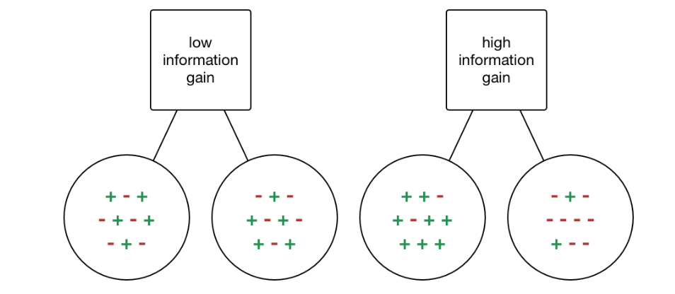
Information Gain (IG) is a metric used to measure the reduction in entropy after splitting a dataset on an attribute. It calculates how well a given attribute separates the training examples according to their target classification. Mathematically, it is defined as:

\[\text{IG}(T, X) = \text{Entropy}(T) - \sum_{j=1}^{K} \frac{|T_j|}{|T|} \text{Entropy}(T_j)\]

where $T$ is the dataset before the split, $T_j$ represents each subset generated by the split, $K$ is the number of subsets, and $\text{Entropy}(T)$ is the entropy of the dataset $T$. Information Gain is maximized when the attribute splits the data into the purest possible sub-groups, reducing overall entropy.

Gini Index

The Gini Index is another metric used to evaluate splits in the dataset, particularly for binary splits. It is defined as the probability of incorrectly classifying a randomly chosen element from the dataset if it were labeled according to the distribution of labels in the subset. The Gini Index for a node $T$ is given by:

\[\text{Gini}(T) = 1 - \sum_{i=1}^{C} p_i^2\]

where $C$ is the number of classes and $p_i$ is the probability of selecting a sample with class $i$. A lower Gini Index indicates higher purity, meaning a more homogeneous subset.

Comparison of Information Gain and Gini Index

Metric	Information Gain	Gini Index
Type of Split	Works best with multiple splits	Generally used for binary splits
Calculation	Based on entropy reduction	Based on probability of misclassification
Range	Non-negative, varies by dataset	Ranges from 0 to 0.5 for binary classification
Preference	Prefers attributes with many distinct values	Often simpler and computationally efficient
Bias	Biased towards attributes with more categories	Less biased towards highly categorical attributes

One-hot encoding of categorical features

If a feature has $k > 2$ categorical values, change the feature to k binary features that have the value of 0 or 1.

Continuous valued features

Choose the $m - 1$ mid-points between the $m$ examples as possible splits, and find the split that gives the highest information gain.

Regression Trees

When choosing a split for a regression tree, we pick the feature with the highest reduction in variance.

\[\overline{x} = \frac{\sum{x}}{n}\] \[{V = \sigma^2 = \frac{\sum{x_i^2} - n\overline{x}}{n - 1}}\] \[\text{Reduction in Variance} = V(\text{root}) - (w^{\text{left}}V(\text{left}) + w^{\text{right}}V(\text{right}))\]

Learning Process

Iterative Process

• All the labeled examples set in a node

• At each node:

  • Calculate information gain for all possible features and pick the one with the highest information gain
  • Split examples according to the selected feature, creating left and right branches of the tree
  • Continue the recursive splitting process until stopping criteria are met

Stopping Criteria

• The examples of a node are completely in the same class
• The tree exceeds the maximum depth
• Information gain from additional splits is less than the threshold
• Number of examples in a node is below the threshold

Random Forest

Tree ensemble

We have the fact that decision tree algorithm highly sensitive to small changes in the data, changing just one training example causes the algorithm to come up with a different split at the root and then a totally different tree. Therefore, to make the algorithm less sensitive or more robust, we will build not just one decision tree, but a group of multiple decision trees, and we call that a tree ensemble.\

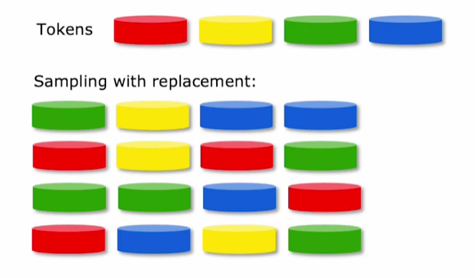
Random forest is an algorithm that we apply tree ensemble, for each tree, the train set is sampled with replacement to create a new train set and features are randomly chosen.

Sampling with replacement train set

In the process of dataset generation for each tree, we apply sampling with replacement, which means after selecting randomly a train sample from the original train set, we put it back into the population then continue with another sample until we get the set of m train samples.

Randomizing the feature choice

In case, we have totally n features, when choosing a feature to split at each node, we pick randomly a subset of $k \leq n$, typically $k = \sqrt{n}$ features and let the algorithm only select a feature from the subset of these k features.

Learning Process

Iterative Process

• Given $m$ training examples and $n$ features

• Loop for a limited number of times (typically ranging from 64 to 128), which is the number of generated trees:

  • Use sampling with replacement to generate a new training set of size $m$
  • Train a decision tree on the new dataset, with each node split by one of $k = \sqrt{n}$ random features
  • The decision tree returns a vote

• The final prediction is:

  • The highest vote for a categorical target
  • The average of votes for a continuous target