Evaluation metrics

Confusion Matrix and Fundamental Metrics

Let’s assume a system aims to detect whether essays are generated by an AI model (e.g., a Large Language Model, LLM) or human-written. A sample of 100 essays is analyzed, and the results are summarized as follows:

• 40 essays are generated by an LLM (positive cases).

• 60 essays are human-written (negative cases).

• The model predicts 45 essays as LLM-generated (positive prediction) and 55 as human-written (negative prediction).

The confusion matrix consists of four fundamental metrics that are used to evaluate the classifier:

• TP (True Positive): The number of correctly classified LLM-generated essays.

• TN (True Negative): The number of correctly classified human-written essays.

• FP (False Positive): The number of human-written essays misclassified as LLM-generated. FP is also known as Type I error.

• FN (False Negative): The number of LLM-generated essays misclassified as human-written. FN is also known as Type II error.

True Positive Rate (TPR) / Recall / Sensitivity

Recall shows the proportion of true positive predictions among all actual positive instances (LLM-generated essays) in the dataset. Here, TPR measures the proportion of actual LLM-generated essays correctly identified.

False Positive Rate (FPR)

FPR shows the proportion of false positives among all actual negative instances (human-written essays). In this case, FPR represents the proportion of human-written essays incorrectly classified as LLM-generated.

Precision (Positive Predictive Value)

Precision measures the ratio of correctly classified LLM-generated essays (TP) to the total number of essays predicted to be LLM-generated (TP+FP).

Accuracy

Accuracy represents the overall proportion of correct predictions.

F1 Score (F Measure)

The F1 score is the harmonic mean of precision and recall, balancing both metrics.

F-beta Score

Evolve from F1 score, F-beta score is also called "weighted harmonic mean of precision and recall", where the parameter $\beta$ controls the balance between precision and recall.

• If FP and FN both are important, $\beta = 1$ (F1 score)

• If FP is more important than FN, $\beta < 1$

• If FN is more important than FP, $\beta > 1$

Classification threshold

It is clear that a probabilistic classification model produces a probability score between 0 (totally human-written) and 1 (totally AI-written) for each essay, indicating the likelihood that it is AI-written. For instance, the model may assign a probability of 0.9 that an essay is AI-written. To determine the actual class label (human or AI), a classification threshold is applied.

• If the threshold is set to 0.5, any essay with a predicted probability above 0.5 is categorized as AI-written (class 1).

• Alternatively, a more conservative threshold of 0.8 might be chosen, only classifying essays with a probability exceeding 0.8 as AI-written.

The choice of classification threshold depends on the specific problem and the costs associated with different error types. For example, in detecting AI-written essays, a false positive (classifying a human-written essay as AI-written) may be less detrimental than a false negative (failing to detect an AI-written essay). In such cases, a lower threshold might be preferred to ensure higher recall, even if it leads to some false positives.

As you change the threshold, you will usually get new combinations of errors of different types (and new confusion matrices).

The selection of the classification threshold influences the model’s error rate. A higher threshold increases the model’s conservatism, assigning the label of AI-written only with greater confidence, but resulting in lower recall by detecting fewer true positive (AI-written) cases. Conversely, a lower threshold makes the model less strict, leading to higher recall, but potentially lower precision due to an increase in false positives (human-written essays classified as AI-written).

Modifying the classification threshold affects both the True Positive Rate (TPR) and False Positive Rate (FPR), causing them to change in the same direction. A higher TPR (recall) typically corresponds to a higher FPR, and vice versa.

Consider the following scenario where the recall (TPR) decreases as the decision threshold is set higher:

• Threshold of 0.5: $\dfrac{800}{800 + 100} = 0.89$ (Recall for AI-written essays)

• Threshold of 0.8: $\dfrac{600}{600 + 300} = 0.67$

• Threshold of 0.95: $\dfrac{200}{200 + 700} = 0.22$

Similarly, the FPR also decreases:

• Threshold of 0.5: $\dfrac{500}{500 + 8600} = 0.06$ (FPR, indicating the rate at which human-written essays are misclassified as AI-written)

• Threshold of 0.8: $\dfrac{100}{100 + 9000} = 0.01$

• Threshold of 0.95: $\dfrac{10}{10 + 9090} = 0.001$

Receiver Operating Characteristic (ROC) curve

The ROC curve was first developed by electrical engineers and radar engineers during World War II for detecting enemy objects in battlefields, starting in 1941, which led to its name ("receiver operating characteristic"). The ROC curve plots the True Positive Rate (TPR) against the False Positive rate (FPR) at various classification thresholds. Revising the previous section, we can derive TPR and FPR from a confusion matrix. The ROC curve is the most popular form of trade-off between TPR and FPR. Unless the model is near-perfect, we have to balance the two. As we try to increase the TPR (i.e., correctly identify more positive cases), the FPR may also increase (i.e., you get more false alarms). The more AI-written essays we want to detect, the more human-written essays which are falsely identified.

The ROC curve is a visual representation of this choice. Each point on the curve corresponds to a combination of TPR and FPR values at a specific decision threshold.

We will plot a ROC curve using scikit-learn’s visualization API, RocCurveDisplay.

import matplotlib.pyplot as plt

from sklearn.datasets import load_wine
from sklearn.ensemble import RandomForestClassifier
from sklearn.metrics import RocCurveDisplay
from sklearn.model_selection import train_test_split
from sklearn.svm import SVC

X, y = load_wine(return_X_y=True)
y = y == 2

X_train, X_test, y_train, y_test = train_test_split(X, y, random_state=42)
svc = SVC(random_state=42)
svc.fit(X_train, y_train)

rfc = RandomForestClassifier(n_estimators=10, random_state=42)
rfc.fit(X_train, y_train)

ax = plt.gca()      # Get the current axis. Prevent the two ROC curves having different axes
svc_disp = RocCurveDisplay.from_estimator(svc, X_test, y_test, ax=ax, alpha=0.8) 
rfc_disp = RocCurveDisplay.from_estimator(rfc, X_test, y_test, ax=ax, alpha=0.8)

plt.show()

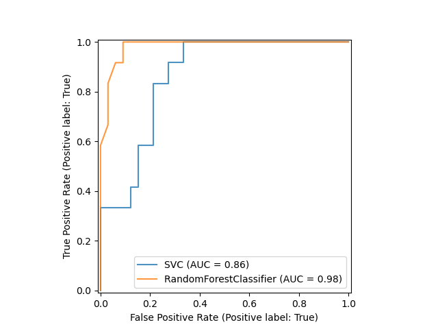
The left side of the curve corresponds to the more "confident" thresholds: a higher threshold leads to lower recall and fewer false positive errors. The extreme point is when both recall and FPR are 0. In this case, there are no correct detections but also no false ones.

The right side of the curve represents the "less strict" scenarios when the threshold is low. Both recall and False Positive rates are higher, ultimately reaching 100%. If you put the threshold at 0, the model will always predict a positive class: both recall, and the FPR will be 1.

When you increase the threshold, you move left on the curve. If you decrease the threshold, you move to the right.

The ROC area under the curve (ROC AUC) is basically the ratio between the area under the curve and the rectangle formed by the TPR and FPR axes.

The perfect scenario would be the model identifying all cases correctly and never giving false alarms.

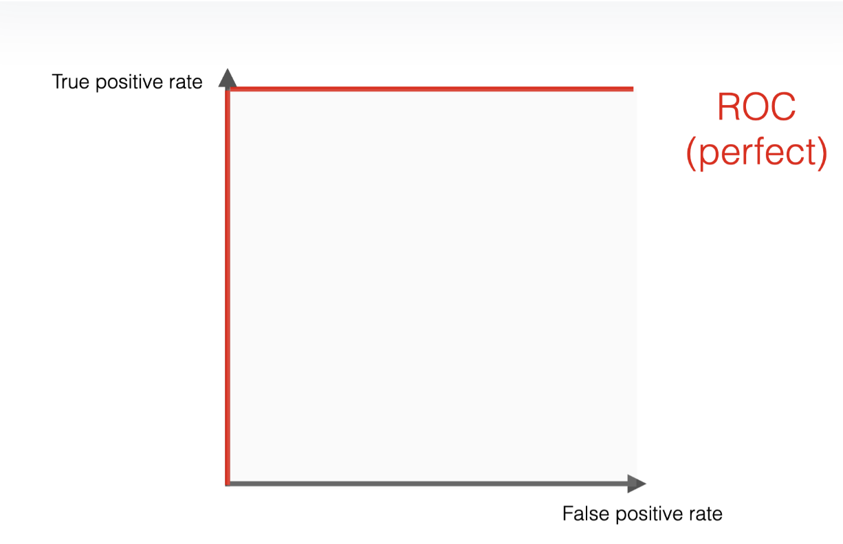
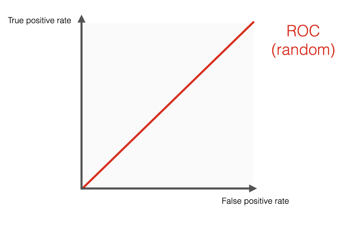
The worst scenario would be our model giving literally random results, leading to the ROC curve begin a diagonal line connecting (0,0) to (1,1). For a random classifier, the TPR is equal to the FPR because it makes the same number of true and false positive predictions for any threshold value. As the classification threshold changes, the TPR goes up or down in the same proportion as the FPR.

import numpy as np

# Generate an array of 100 points
y_true = np.random.randint(0, 2, size=100)  # 100 true labels (0 or 1)
y_scores = np.random.rand(100)  # 100 random scores between 0 and 1

import matplotlib.pyplot as plt

from sklearn.datasets import load_wine
from sklearn.ensemble import RandomForestClassifier
from sklearn.metrics import RocCurveDisplay, auc, roc_curve
from sklearn.model_selection import train_test_split
from sklearn.svm import SVC

fpr, tpr, _ = roc_curve(y_true, y_scores)
roc_auc = auc(fpr, tpr)

# Create ROC Curve plot
roc_display = RocCurveDisplay(fpr=fpr, tpr=tpr, roc_auc=roc_auc, estimator_name='Example Model')

# Plot and save
roc_display.plot()
plt.savefig('ROC AUC random.png')  # Save the ROC curve plot as an image

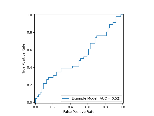
Most real-world models will fall somewhere between the two extremes. The better the model can distinguish between positive and negative classes, the closer the curve is to the top left corner of the graph. As a rule of thumb, a ROC AUC score above 0.8 is considered good, while a score above 0.9 is considered great.

Evaluation

The intuition behind ROC AUC is that it measures how well a binary classifier can distinguish or separate between the positive and negative classes. It reflects the probability that the model will correctly rank a randomly chosen positive instance higher than a random negative one.

ROC AUC is a powerful metric for evaluating binary classification models. However, its usefulness depends on the context and the specific goals of your model.

When to Use ROC AUC:

• Comparing Multiple Models: ROC AUC is valuable during model training to compare the overall performance of multiple models. Since it summarizes the performance across different thresholds in a single number, it is easy to use when you want to identify the best-performing model in general terms.

• Ranking Predictions by Confidence: If your primary goal is to rank predictions by how confident the model is, rather than making hard predictions at a fixed threshold, ROC AUC is ideal. It measures how well the model separates the positive class from the negative class, regardless of the decision threshold.

• Model Monitoring in Production: During production model monitoring, ROC AUC can track whether the model still separates positive and negative classes effectively, especially when class distributions change over time. This can provide an early warning of deteriorating model performance before more granular metrics like precision and recall are impacted.

When Not to Use ROC AUC:

Considering the imbalanced nature of our dataset (too many human-written essays compared to AI-written), and that they have equal importance to the model, the F1-score is the best choice amongst the given metrics.

More info about why ROC AUC is insufficient for imbalanced dataset:

https://www.kaggle.com/code/lct14558/imbalanced-data-why-you-should-not-use-roc-curve

Type I Error vs Type II Error: An Inevitable Tradeoff

Type I and Type II errors play critical roles in various fields, including law and medicine, where the consequences of each error can significantly impact lives and society. Let’s explore the tradeoffs and implications in these domains.

Case study 1: Law

• Type I Error (False Positive): Convicting an innocent person, also known as a "false conviction."

• Type II Error (False Negative): Failing to convict a guilty person, often referred to as a "false acquittal."

Implications of Type I Errors: A Type I error in law undermines trust in the justice system, as it leads to wrongful punishment. An innocent person suffers loss of freedom, reputation, and often mental well-being, and society bears the cost of their wrongful incarceration.

Implications of Type II Errors: A Type II error lets a guilty person go free, potentially endangering society by allowing harmful individuals to re-offend. It can also diminish the perceived deterrent effect of the justice system.

Most legal systems operate under the principle that "it is better that ten guilty persons escape than one innocent suffer." This reflects a strong preference to avoid Type I errors, prioritizing the protection of innocent individuals over convicting the guilty.

Lie detectors are sometimes used in criminal investigations, and both errors can have significant consequences:

• Type I Error (False Positive): An honest person is falsely labeled as lying, leading to suspicion or investigation.

• Type II Error (False Negative): A deceptive individual is classified as truthful, potentially hindering justice.

Implications of Type I Error: False positives in lie detection can lead to unnecessary legal pressure on innocent individuals, potentially affecting mental health and biasing judicial outcomes.

Implications of Type II Error: False negatives allow deceptive individuals to avoid detection, potentially hindering the pursuit of justice.

Often, there is a preference to avoid Type I errors to prevent wrongful suspicion of innocent individuals.

Case study 2: Medicine

In medicine, Type I and Type II errors relate to the diagnosis and treatment of diseases, where both types of errors can have serious consequences:

• Type I Error (False Positive): Diagnosing a patient with a condition they do not have, leading to unnecessary treatment.

• Type II Error (False Negative): Failing to diagnose a condition that is actually present, resulting in a lack of necessary treatment.

Implications of Type I Errors: A Type I error may lead to unnecessary treatments, side effects, psychological stress, and medical costs. For instance, diagnosing a patient with cancer who doesn’t have it can lead to anxiety and harmful treatments.

Implications of Type II Errors: A Type II error may delay treatment, worsening the patient’s condition and potentially reducing recovery chances. For example, failing to diagnose cancer early can make the disease harder to treat or even fatal.

In cases of life-threatening conditions (e.g., cancer, heart disease), doctors often prioritize avoiding Type II errors to ensure early detection, tolerating more false positives (Type I errors) as a result.

Case study 3: AI in Academic Research Preference Against Type I Error: There may be a preference to avoid Type I errors to protect researchers from undue scrutiny, given the reputational risks.

Implications of Type I Error: False positives may discourage researchers from using advanced tools or even language assistance that could be mistakenly flagged, limiting their productivity or creativity.

Implications of Type II Error: False negatives, however, can allow academic misconduct to go undetected. When AI-generated content is mistakenly classified as human-written, it can lead to an erosion of academic standards, as well as skewed or unreliable research findings, particularly if such content is submitted as original work or influences peer-reviewed research.

Preference Against Type I Error: In many academic contexts, there may be a preference to avoid Type I errors to protect innocent researchers from undue scrutiny or accusations. Labeling a human-authored work as AI-generated can lead to distrust in the detection system and harm honest researchers’ reputations. However, excessive Type II errors could undermine research integrity if AI-generated work is mistaken for human-authored content.

Impossibility Results for Reliable Detection of AI-Generated Text

In probability theory, the total variation distance is a distance measure for probability distributions. It is an example of a statistical distance metric and is sometimes called the statistical distance, statistical difference or variational distance.

Definition

Consider a measurable space $(\Omega, \mathcal{F})$ and probability measures $P$ and $Q$ defined on $(\Omega, \mathcal{F})$. The total variation distance between $P$ and $Q$ is defined as \(\delta(P, Q) = \sup_{A \in \mathcal{F}} |P(A) - Q(A)|.\) This is the largest absolute difference between the probabilities that the two probability distributions assign to the same event.

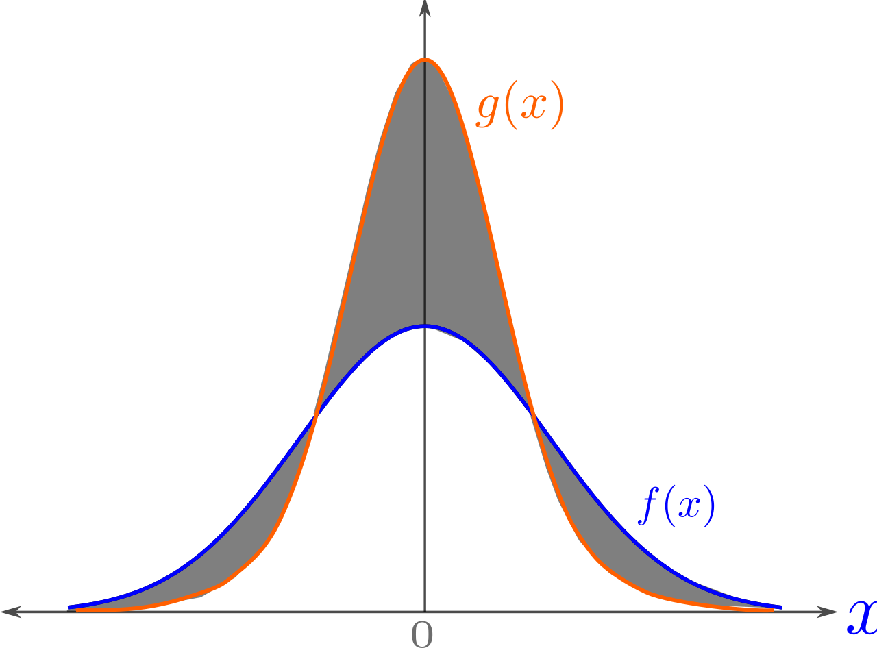
In the following theorem, we formalize the above statement by showing an upper bound on the area under the ROC curve of an arbitrary detector in terms of the total variation distance between the distributions for AI and human-generated text. This bound indicates that as the distance between these distributions diminishes, the ROC AUC bound approaches $1/2$, which represents the baseline performance corresponding to a detector that randomly labels text as AI or human-generated. We define $\mathcal{M}$ and $\mathcal{H}$ as the text distributions produced by an AI model and humans, respectively, over the set of all possible text sequences $\Omega$. We use $TV(\mathcal{M}, \mathcal{H})$ to denote the total variation distance between these two distributions and a function $D : \Omega \rightarrow \mathbb{R}$ that maps every sequence in $\Omega$ to a real number. Sequences are classified into AI and human-generated by applying a threshold $\gamma$ on this number. By adjusting the parameter $\gamma$, we can tune the sensitivity of the detector to AI and human-generated texts to obtain an ROC curve.

Theorem 1. The area under the ROC of any detector $D$ is bounded as

Proof. The ROC is a plot between the true positive rate (TPR) and the false positive rate (FPR) which are defined as follows:

and

where $\gamma$ is some classifier parameter. We can bound the difference between the $\text{TPR}\gamma$ and the $\text{FPR}\gamma$ by the total variation between $\mathcal{M}$ and $\mathcal{H}$:

Since the $\text{TPR}_\gamma$ is also bounded by 1 we have:

Denoting $\text{FPR} _ \gamma$, $\text{TPR} _ \gamma$, and

$TV(\mathcal{M}, \mathcal{H})$ with $x$, $y$, and $tv$ for brevity, we bound the ROC AUC as follows:

$\square$

For a detector to have a good performance (say, $ROC AUC \ge 0.9$), the distributions of human and AI-generated texts must be very different from each other (total variation > 0.5). As the two distributions become similar (say, $total variation \le 0.2$), the performance of even the bestpossible detector is not good ($ROC AUC < 0.7$). This shows that distinguishing the text produced by a language model from a human-generated one is a fundamentally difficult task.

In a recent paper, Feizi analyzed two types of errors that affect the reliability of AI text detectors: type I errors, where human-written text is mistakenly identified as AI-generated, and type II errors, where AI-generated text goes undetected.

Feizi, who holds a joint appointment at the University of Maryland Institute for Advanced Computer Studies, pointed out that commonly available tools like paraphrasers can contribute to type II errors by altering AI-generated text in a way that allows it to evade detection. A notable example of a type I error recently gained attention online when AI detection software incorrectly flagged the U.S. Constitution as AI-generated, underscoring the potential for such technology to make glaring mistakes.

These errors can have serious consequences. Mistakes made by AI detectors can be especially damaging when used by authorities like educators or publishers, who may accuse students and other creators of using AI when, in fact, their work is original. Such accusations are often difficult to dispute, and when proven false, they can damage the reputations of the companies and developers behind the faulty AI detectors. Additionally, even large language models (LLMs) protected by watermarking schemes remain vulnerable to spoofing attacks, where malicious actors can infer hidden watermarks and add them to human-created text, causing it to be incorrectly flagged as AI-generated. These risks, Feizi argues, highlight the need for caution in relying solely on AI detectors to verify the authenticity of human-created content.

Feizi further emphasized the fundamental limitations of these detectors. He explained that, theoretically, it is impossible to reliably determine whether a random sentence was written by a human or generated by AI, given the close similarity in distribution between human and AI-generated content. This challenge is compounded by the sophistication of modern LLMs and the tools available to circumvent detection, like paraphrasers or spoofing techniques.

Our experiments show that paraphrasing the LLM outputs helps evade these detectors effectively. Moreover, our theory demonstrates that for a sufficiently advanced language model, even the best detector can only perform marginally better than a random classifier. This means that for a detector to have both low type-I and type-II errors, it will have to trade off the LLM’s performance.

The line between human and AI-generated content is becoming increasingly blurred due to these variables, Feizi noted, and there is an inherent upper limit to the effectiveness of AI detectors. Consequently, he argues, it is unlikely that highly reliable detectors for AI-generated content will be developed in the foreseeable future.