Decision Tree

Overview

The Decision Tree algorithm is a supervised learning method capable of handling both classification and regression tasks. It works by learning decision rules inferred from the training data to predict the target variable’s value or class. Starting from the root, the algorithm sorts records down the tree based on attribute comparisons until reaching a terminal node that represents the prediction.

Types of Decision Trees

Decision trees are classified by the type of target variable:

• Categorical Variable Decision Tree: Used when the target variable is categorical.

• Continuous Variable Decision Tree: Used for continuous target variables.

Important Terminology

• Root Node: Represents the complete dataset, divided into sub-nodes.

• Splitting: Dividing a node into sub-nodes.

• Decision Node: A node that splits into further sub-nodes.

• Leaf/Terminal Node: A node with no further splits.

• Pruning: The process of removing sub-nodes to avoid overfitting.

• Branch/Sub-Tree: A sub-section of the entire tree.

• Parent and Child Nodes: The parent node divides into child nodes.

Working Mechanism of Decision Trees

Decision Trees work by making strategic splits based on attributes that maximize homogeneity in the sub-nodes. Multiple algorithms guide this splitting process, including:

• ID3 (Iterative Dichotomiser 3): Selects attributes with the highest information gain.

• C4.5: Successor of ID3, uses gain ratio to overcome information gain bias.

• CART (Classification and Regression Tree): Uses the Gini index for classification and regression tasks.

• CHAID (Chi-square Automatic Interaction Detection): Uses Chi-square tests for classification trees.

• MARS (Multivariate Adaptive Regression Splines): Useful for regression tasks.

Attribute Selection Measures

Selecting the root and internal nodes is based on attribute selection measures like:

• Entropy and Information Gain: Used to calculate the reduction in entropy before and after a split.

• Gini Index: Measures impurity for binary splits.

• Gain Ratio: Adjusts information gain for attributes with many distinct values.

• Reduction in Variance: Useful for continuous target variables.

• Chi-Square: Evaluates statistical significance in splits.

Overfitting and Pruning

Decision trees are prone to overfitting when they are too complex. Overfitting can be countered by:

• Pruning: Trimming branches that add little predictive power.

• Random Forest: An ensemble method that builds multiple trees using random subsets of the data and features, reducing overfitting by averaging the predictions.

Information Gain

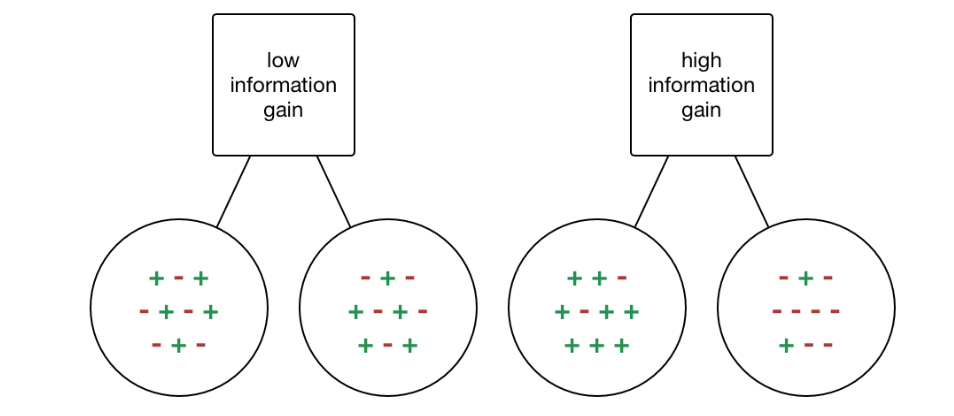
Information Gain (IG) is a metric used to measure the reduction in entropy after splitting a dataset on an attribute. It calculates how well a given attribute separates the training examples according to their target classification. Mathematically, it is defined as:

\[\text{IG}(T, X) = \text{Entropy}(T) - \sum_{j=1}^{K} \frac{|T_j|}{|T|} \text{Entropy}(T_j)\]

where $T$ is the dataset before the split, $T_j$ represents each subset generated by the split, $K$ is the number of subsets, and $\text{Entropy}(T)$ is the entropy of the dataset $T$. Information Gain is maximized when the attribute splits the data into the purest possible sub-groups, reducing overall entropy.

Gini Index

The Gini Index is another metric used to evaluate splits in the dataset, particularly for binary splits. It is defined as the probability of incorrectly classifying a randomly chosen element from the dataset if it were labeled according to the distribution of labels in the subset. The Gini Index for a node $T$ is given by:

\[\text{Gini}(T) = 1 - \sum_{i=1}^{C} p_i^2\]

where $C$ is the number of classes and $p_i$ is the probability of selecting a sample with class $i$. A lower Gini Index indicates higher purity, meaning a more homogeneous subset.

Comparison of Information Gain and Gini Index

Metric	Information Gain	Gini Index
Type of Split	Works best with multiple splits	Generally used for binary splits
Calculation	Based on entropy reduction	Based on probability of misclassification
Range	Non-negative, varies by dataset	Ranges from 0 to 0.5 for binary classification
Preference	Prefers attributes with many distinct values	Often simpler and computationally efficient
Bias	Biased towards attributes with more categories	Less biased towards highly categorical attributes