Perceptron Learning Algorithm

Problem Statement

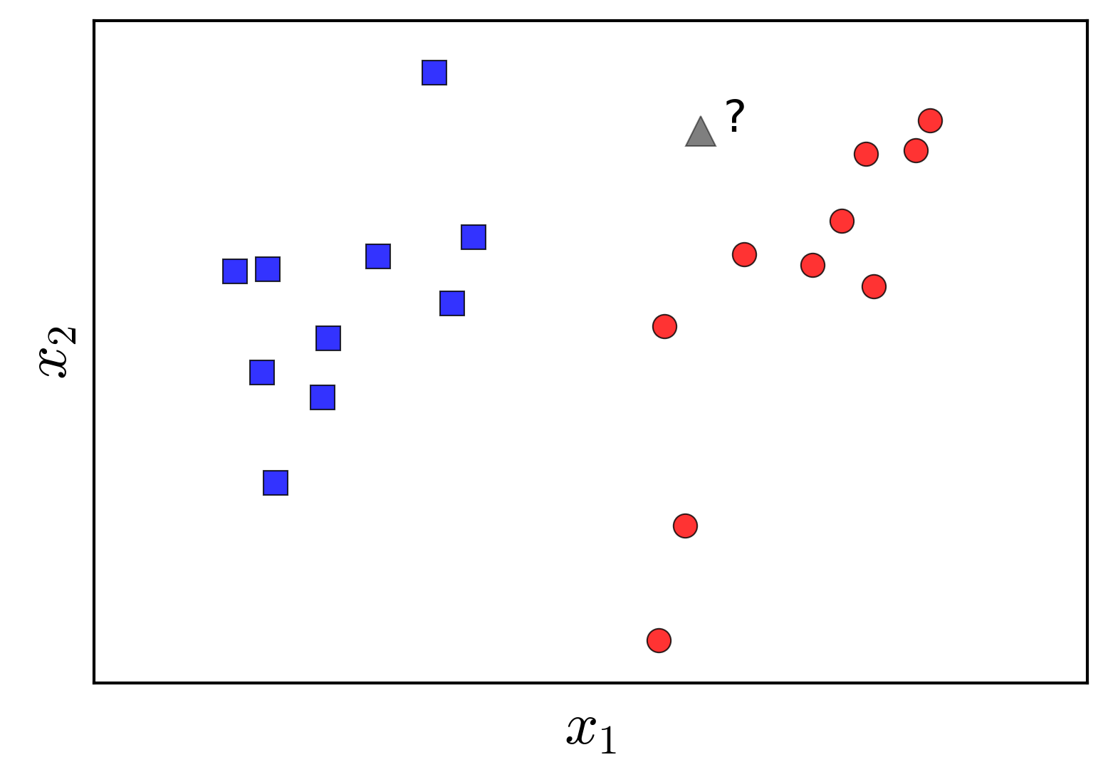
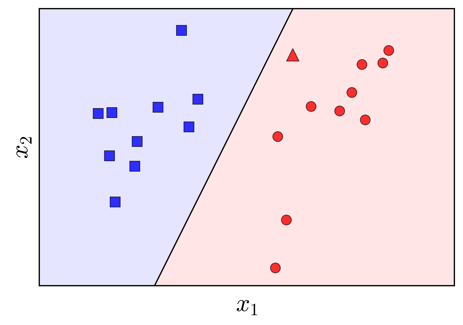
Consider two labeled datasets, represented visually in Figure$~\ref{fig:1}$ on the left. The two classes in this example are represented by blue and red points. The objective is to construct a classifier that can predict the label of a new data point (illustrated as a grey triangle), given the labeled data of the two classes.

The Perceptron problem can be formally stated as follows: Given two labeled classes, find a linear boundary such that all points belonging to class 1 lie on one side of the boundary, and all points belonging to class 2 lie on the opposite side. Assume that such a linear boundary exists.

When such a boundary exists, the two classes are said to be linearly separable. Classification algorithms that construct linear boundaries are commonly referred to as linear classifiers.

Much like other iterative algorithms such as Gradient Descent, the basic idea behind PLA is to start with an initial guess for the boundary and iteratively improve it. At each iteration, the boundary is updated to move closer to an optimal solution. This update process is driven by minimizing a loss function that quantifies the misclassification error.

Notation

Let us denote the matrix of data points as

$\mathbf{X} = [\mathbf{x}_1, \mathbf{x}_2, \dots, \mathbf{x}_N] \in \mathbb{R}^{d \times N}$,

where each column $\mathbf{x}_i \in \mathbb{R}^{d \times 1}$ represents a data point in $d$-dimensional space. (Note: data points are represented as column vectors for convenience)

Assume that the corresponding labels are stored in a row vector

$\mathbf{y} = [y_1, y_2, \dots, y_N] \in \mathbb{R}^{1 \times N}$,

where

$y_i = 1$ if $\mathbf{x}_i$ belongs to class 1 (blue), and $y_i = -1$ if $\mathbf{x}_i$ belongs to class 2 (red).

At any given point in the algorithm, suppose we have identified a linear boundary, which can be described by the equation:

\[\begin{aligned} f_{\mathbf{w}}(\mathbf{x}) &= w_1 x_1 + \dots + w_d x_d + w_0 = \mathbf{w}^T \mathbf{\bar{x}} = 0 \end{aligned}\]

where $\mathbf{w} \in \mathbb{R}^{d+1}$ is the weight vector, and $\mathbf{\bar{x}} = [x_1, x_2, \dots, x_d, 1]^T \in \mathbb{R}^{d+1}$ is the augmented data point (including a bias term).

With $\mathbf{\bar{x}}$, we denote the extended data point by adding an element $x_0 = 1$ to the beginning of the vector $\mathbf{x}$, similar to the method used in linear regression. Henceforth, we will assume that $\mathbf{x}$ refers to the extended data point.

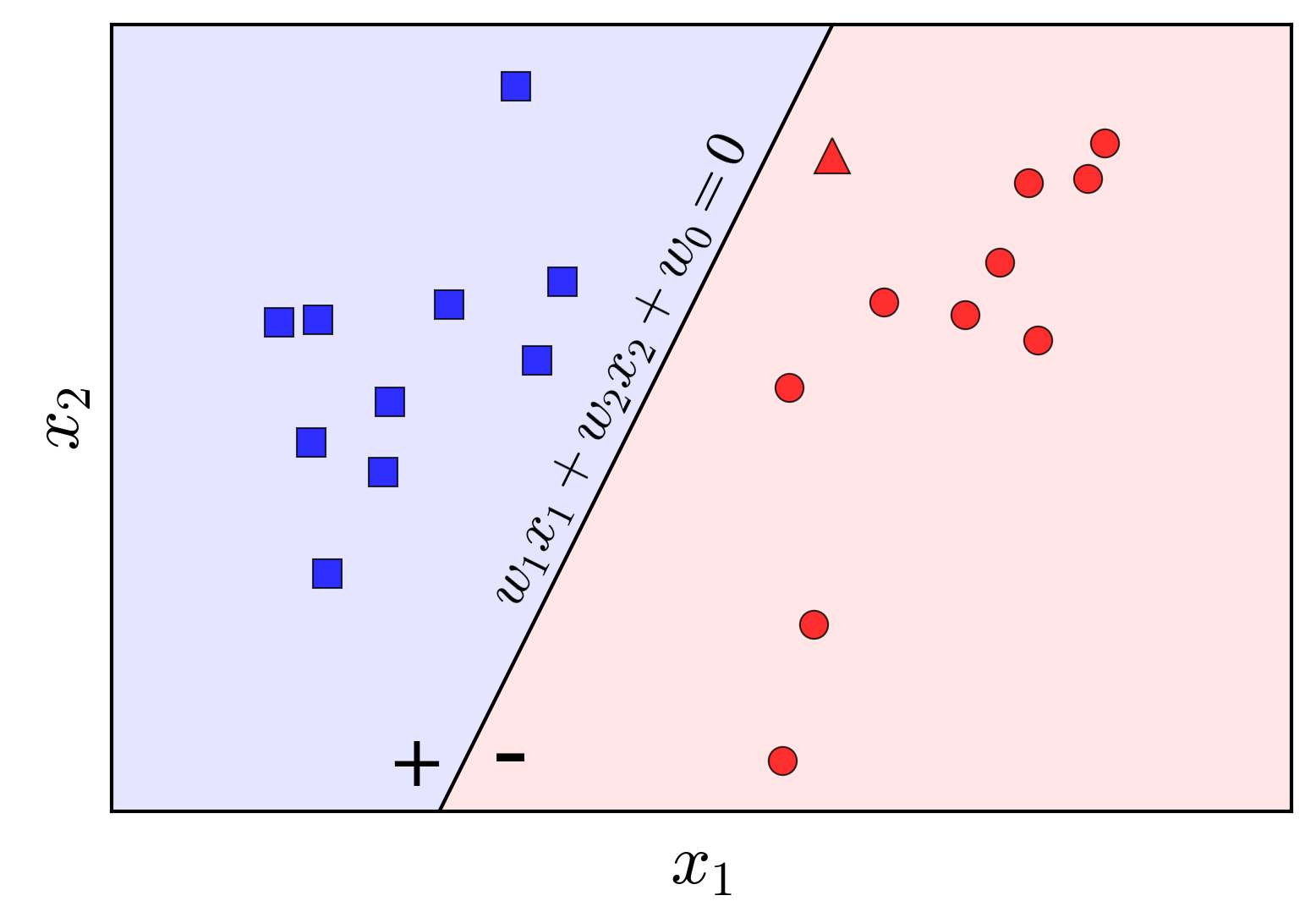
For simplicity, let us consider the case where each data point has two dimensions, i.e., $d = 2$. Suppose the line equation $w_1 x_1 + w_2 x_2 + w_0 = 0$ represents the solution we seek, as shown in Figure$~\ref{fig:2}$:

We observe that points lying on the same side of this line will have the same sign for the function $f_{\mathbf{w}}(\mathbf{x})$. By adjusting the sign of $\mathbf{w}$ as necessary, we assume that points on the positive side of the line (the blue-shaded half-plane) have positive labels (+), while points on the negative side (the red-shaded half-plane) have negative labels (-). These signs correspond to the label $y$ for each class. Thus, if $\mathbf{w}$ is a solution to the Perceptron problem, for a new unlabeled data point $\mathbf{x}$, we can determine its class by a simple computation:

\[\begin{aligned} \text{label}(\mathbf{x}) &=& 1 \quad\text{if} \quad \mathbf{w}^T\mathbf{x} \geq 0, \nonumber \\ &=& -1 \quad \text{otherwise} \nonumber \end{aligned}\]

In summary:

\[\text{label}(\mathbf{x}) = \text{sgn}(\mathbf{w}^T\mathbf{x})\]

where $\textit{sgn}$ denotes the sign function, and we assume that $\text{sgn}(0) = 1$.

Loss Function Construction

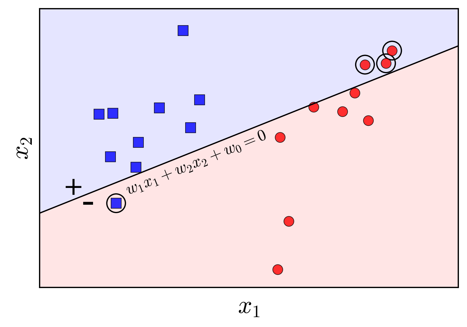
Next, we need to define a loss function for any given parameter $\mathbf{w}$. Still operating in two-dimensional space, assume the line $w_1 x_1 + w_2 x_2 + w_0 = 0$ is given, as illustrated in Figure 3:

In this case, the circled points represent the misclassified data points. Our goal is to have no misclassified points. The simplest loss function we might consider is one that counts the number of misclassified points and seeks to minimize this number:

\[J_1(\mathbf{w}) = \sum_{\mathbf{x}_i \in \mathcal{M}} (-y_i\text{sgn}(\mathbf{w}^T\mathbf{x_i}))\]

where $\mathcal{M}$ is the set of misclassified points (changes relatively to $\mathbf{w}$). For each point $\mathbf{x}_i \in \mathcal{M}$, since the point is misclassified, $y_i$ and $\text{sgn}(\mathbf{w}^T\mathbf{x_i})$ differ, and thus $-y_i\text{sgn}(\mathbf{w}^T\mathbf{x_i}) = 1$. Therefore, $J_1(\mathbf{w})$ is a count of the number of misclassified points. When this function reaches its minimum value of 0, no points are misclassified.

However, an important drawback of this function is that it is discrete and non-differentiable with respect to $\mathbf{w}$, making it challenging to optimize. We require a different loss function that is more amenable to optimization.

Consider the following loss function:

$J(\mathbf{w}) = \sum_{\mathbf{x}_i \in \mathcal{M}} (-y_i\mathbf{w}^T\mathbf{x_i})$

This function differs from $J_1()$ by omitting the $\text{sgn}$ function. Note that for a misclassified point $\mathbf{x}_i$, the further it is from the boundary, the larger the value of $-y_i\mathbf{w}^T\mathbf{x_i}$, indicating a greater degree of error. The minimum value of this loss function is also 0, achieved when no points are misclassified. This loss function is considered superior to $J_1()$ because it penalizes points that are deeply misclassified more heavily, whereas $J_1()$ penalizes all misclassified points equally (with a value of 1), regardless of their proximity to the boundary.

At any given time, if we focus only on the misclassified points, the function $J(\mathbf{w})$ is differentiable. Consequently, we can employ optimization techniques such as Gradient Descent or Stochastic Gradient Descent (SGD) to minimize this loss function. Given the advantages of SGD in large-scale problems, we will follow this approach.

For a single misclassified data point $\mathbf{x}_i$, the loss function becomes:

$J(\mathbf{w}; \mathbf{x}_i; y_i) = -y_i\mathbf{w}^T\mathbf{x}_i$

The corresponding gradient is:

$\nabla_{\mathbf{w}}J(\mathbf{w}; \mathbf{x}_i; y_i) = -y_i\mathbf{x}_i$

Thus, the update rule is:

\[\mathbf{w} = \mathbf{w} + \eta y_i\mathbf{x}_i\]

where $\eta$ is the learning rate, typically set to 1.

This results in a concise update rule: $\mathbf{w}_{t+1} = \mathbf{w}_t + y_i\mathbf{x}_i$. In other words, for each misclassified point $\mathbf{x}_i$, we multiply the point by its label $y_i$ and add the result to $\mathbf{w}$, obtaining the updated weight vector.

We observe the following:

\[\mathbf{w}_{t+1}^T\mathbf{x}_i = (\mathbf{w}_t + y_i\mathbf{x}_i)^T\mathbf{x}_i = \mathbf{w}_t^T\mathbf{x}_i + y_i \|\mathbf{x}_i\|_2^2\]

If $y_i = 1$, since \(\mathbf{x}_i\) is misclassified, \(\mathbf{w}_t^T\mathbf{x}_i < 0\). Additionally, since \(y_i = 1\), we have

\(y_i \|\mathbf{x}_i\|_2^2 = \|\mathbf{x}_i\|_2^2 \geq 1\) (note that \(x_0 = 1\)), which implies that \(\mathbf{w}_{t+1}^T\mathbf{x}_i > \mathbf{w}_t^T\mathbf{x}_i\). This means that \(\mathbf{w}_{t+1}\) moves toward correctly classifying \(\mathbf{x}_i\). A similar argument applies when \(y_i = -1\).

Thus, our intuition for this algorithm is as follows: pick a boundary, and for each misclassified point, move the boundary towards correctly classifying that point. Although previously correctly classified points may become misclassified during this process, the Perceptron Learning Algorithm (PLA) is guaranteed to converge after a finite number of steps (we will not elaborate further on the proof). In other words, we will eventually find a hyperplane that separates the two classes, provided that they are linearly separable.

Summary

The Perceptron Learning Algorithm can be summarized as follows:

1. Initialize the weight vector $\mathbf{w}$ with values close to zero.

2. Randomly iterate through each data point $\mathbf{x}_i$:

   • If $\mathbf{x}_i$ is correctly classified, i.e., $\text{sgn}(\mathbf{w}^T\mathbf{x}_i) = y_i$, do nothing.

   • If $\mathbf{x}_i$ is misclassified, update $\mathbf{w}$ using the rule: $\mathbf{w} = \mathbf{w} + \eta y_i\mathbf{x}_i$

3. Check how many points remain misclassified. If none, stop the algorithm. Otherwise, repeat from step 2.