Convex Functions

Definition

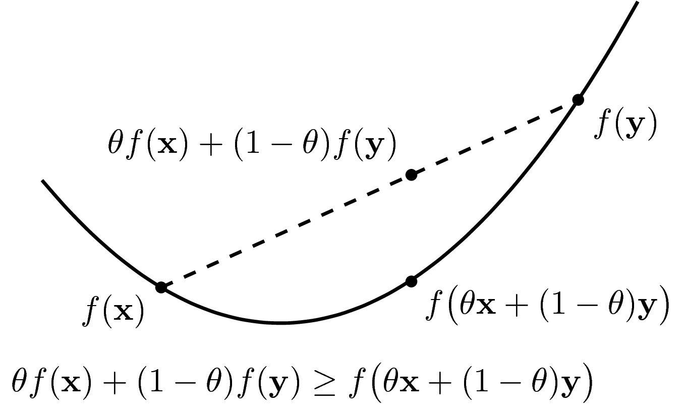
To build an intuitive understanding, let us first examine one-dimensional functions, where the graph of the function is a curve in a plane. A function is called convex if its domain is a convex set, and for any two points on the graph, the line segment connecting them lies above or on the graph itself (refer to Figure 1).

The domain of a function \(f(.)\) is denoted as \(\text{dom} f\).

Definition
A function \(f: \mathbb{R}^n \rightarrow \mathbb{R}\) is called a convex function if \(\text{dom} f\) is a convex set, and for all \(\mathbf{x, y} \in \text{dom} f\) and \(0 \leq \theta \leq 1\),

\[f(\theta \mathbf{x} + (1 - \theta) \mathbf{y}) \leq \theta f(\mathbf{x}) + (1 - \theta) f(\mathbf{y}).\]

The condition that \(\text{dom} f\) is convex is crucial because, without it, we cannot define \(f(\theta \mathbf{x} + (1 - \theta) \mathbf{y})\).

A function \(f\) is called concave if \(-f\) is convex. A function can be neither convex nor concave. Linear functions are both convex and concave.

Definition
A function \(f: \mathbb{R}^n \rightarrow \mathbb{R}\) is called strictly convex if \(\text{dom} f\) is convex, and for all \(\mathbf{x, y} \in \text{dom} f\), \(\mathbf{x} \neq \mathbf{y}\), and \(0 < \theta < 1\), \[f(\theta \mathbf{x} + (1 - \theta) \mathbf{y}) < \theta f(\mathbf{x}) + (1 - \theta) f(\mathbf{y}).\]

Similarly, a function is called strictly concave if \(-f\) is strictly convex.

An important note: If a function is strictly convex and has an extremum, that extremum is unique and is also the global minimum.

Basic Properties

• If \(f(\mathbf{x})\) is convex, then \(af(\mathbf{x})\) is convex if \(a > 0\), and concave if \(a < 0\). This follows directly from the definition.
• The sum of two convex functions is convex, with the domain being the intersection of their domains (the intersection of two convex sets is also convex).
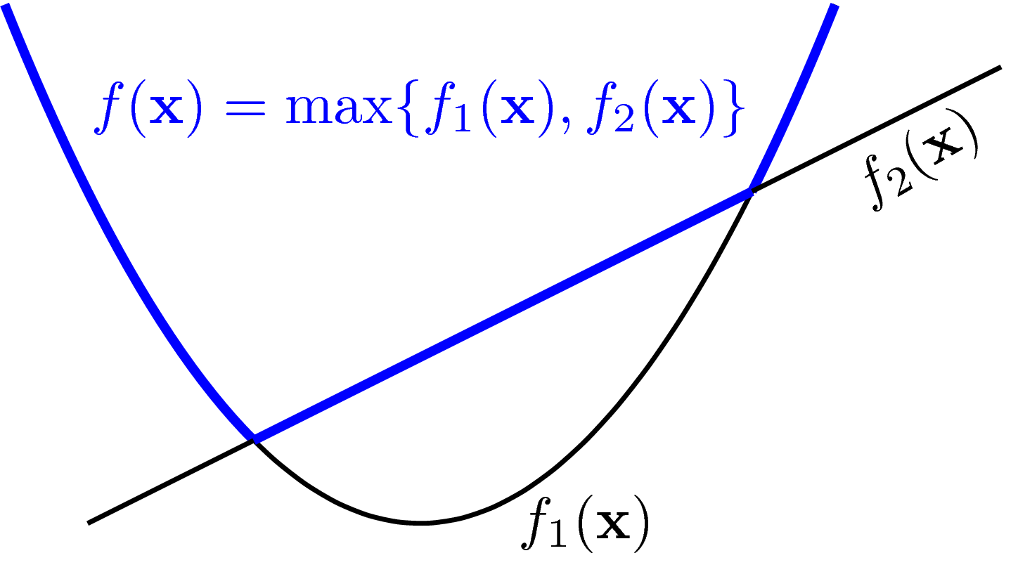
• Pointwise Maximum and Supremum: If the functions \(f_1, f_2, \dots, f_m\) are convex, then \(f(\mathbf{x}) = \max\{f_1(\mathbf{x}), f_2(\mathbf{x}), \dots, f_m(\mathbf{x})\}\) is also convex, where the domain is the intersection of all the domains of the functions. The maximum can also be replaced by the supremum. This property can be proven using the definition of convexity, as illustrated by Figure 2.

Examples

One-variable Functions

Examples of convex one-variable functions include:

• The function \(y = ax + b\) is convex because the line segment between any two points lies on the graph itself.
• The exponential function \(y = e^{ax}\) for any \(a \in \mathbb{R}\).
• The power function \(y = x^a\) on the domain of positive real numbers, for \(a \geq 1\) or \(a \leq 0\).
• The negative entropy function \(y = x \log x\) on the domain of positive real numbers.

Examples of concave one-variable functions include:

• The function \(y = ax + b\) is concave since \(-y\) is convex.
• The power function \(y = x^a\) on the domain of positive real numbers for \(0 \leq a \leq 1\).
• The logarithmic function \(y = \log(x)\) on the domain of positive real numbers.

Affine Functions

Affine functions of the form \(f(\mathbf{x}) = \mathbf{a}^T \mathbf{x} + b\) are both convex and concave.

When the variable is a matrix \(\mathbf{X}\), affine functions take the form: \[f(\mathbf{X}) = \text{trace}(\mathbf{A}^T \mathbf{X}) + b\]

where \(\text{trace}\) denotes the sum of the diagonal elements of a square matrix, and \(\mathbf{A}\) is a matrix of the same dimension as \(\mathbf{X}\) (ensuring matrix multiplication is well-defined).

Quadratic Forms

A quadratic function of the form \(f(x) = ax^2 + bx + c\) is convex if \(a > 0\) and concave if \(a < 0\).

For a vector \(\mathbf{x} = [x_1, x_2, \dots, x_n]\), a quadratic form takes the form: \[f(\mathbf{x}) = \mathbf{x}^T \mathbf{A} \mathbf{x} + \mathbf{b}^T \mathbf{x} + c\]

where \(\mathbf{A}\) is typically a symmetric matrix (i.e., \(a_{ij} = a_{ji}\) for all \(i, j\)), and \(\mathbf{b}\) is a matrix of the same dimension as \(\mathbf{x}\).

If \(\mathbf{A}\) is positive semidefinite, then \(f(\mathbf{x})\) is convex. If \(\mathbf{A}\) is negative semidefinite, \(f(\mathbf{x})\) is concave.

The loss function in Linear Regression has the form:
\[\mathcal{L}(\mathbf{w}) = \dfrac{1}{2} |\mathbf{y} - \mathbf{X} \mathbf{w}|_2^2 = \dfrac{1}{2} (\mathbf{y} - \mathbf{X} \mathbf{w})^T (\mathbf{y} - \mathbf{X} \mathbf{w})\]
Since \(\mathbf{X}^T \mathbf{X}\) is positive semidefinite, the loss function of Linear Regression is a convex function.

Norms

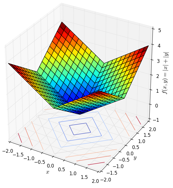
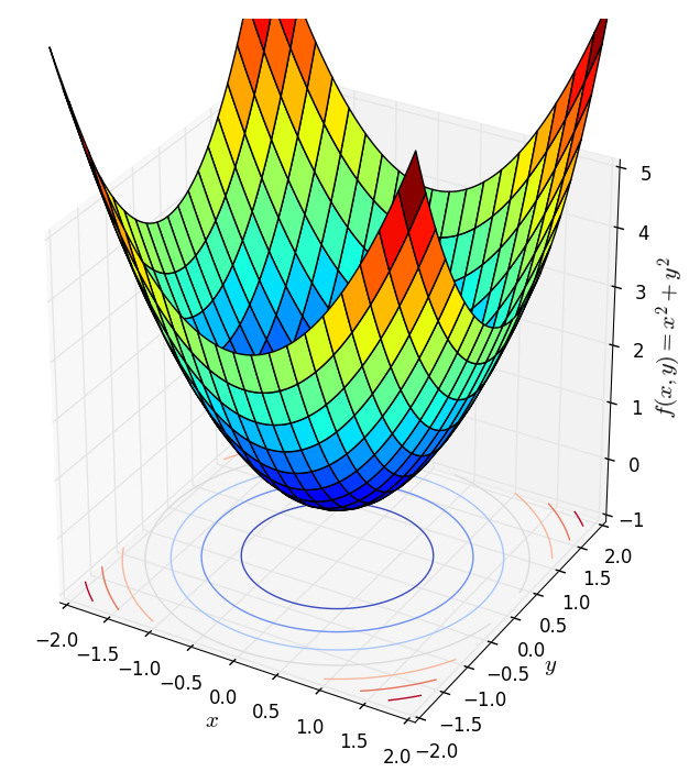
Norms, which satisfy the three conditions of a norm, are also convex functions. Below are examples of the 1-norm (left) and 2-norm (right) with two variables:

These surfaces exhibit a unique bottom corresponding to the origin, a characteristic of strictly convex functions.

\(\alpha\) - sublevel sets

Definition: An \(\alpha\)-sublevel set of a function \(f : \mathbb{R}^n \to \mathbb{R}\) is defined as: \[\mathcal{C}_{\alpha} = \left\{ \mathbf{x} \in \text{dom} f ~\big|~ f(\mathbf{x}) \leq \alpha \right\}\]

That is, the set of points in the domain of \(f\) where \(f\) takes values less than or equal to \(\alpha\).

Referring back to Figure 2, the \(\alpha\)-sublevel sets correspond to the areas enclosed by the level sets.

In the bottom left image, the \(\alpha\)-sublevel sets are the half-plane areas defined by the level lines. In the