Gradient Boosting

Overview and History

Gradient Boosting is a powerful machine learning technique that constructs predictive models by sequentially adding weak learners, typically decision trees, to minimize a specified loss function. This approach improves model accuracy by correcting the errors made by previous learners through an iterative process. Gradient Boosting was introduced by Jerome Friedman in 1999 and has become foundational for regression, classification, and ranking tasks.

The concept of Gradient Boosting originated from the observation by Leo Breiman that boosting can be interpreted as an optimization algorithm on a cost function. This led to the development of explicit regression Gradient Boosting algorithms by Friedman, along with the more general functional gradient boosting perspective introduced by Mason, Baxter, Bartlett, and Frean. Their work viewed boosting algorithms as iterative functional gradient descent algorithms in function space. Gradient Boosting generalizes the concept by optimizing arbitrary differentiable loss functions, allowing for broad applications beyond regression, including classification and ranking problems.

Loss Function

The loss function in Gradient Boosting defines the error or residual to be minimized at each iteration. Different loss functions can be chosen for various tasks, influencing the model’s sensitivity to outliers and overall accuracy.

Regression

In regression tasks, common loss functions include:

• Mean Squared Error (MSE): This loss function is the average squared difference between the predicted and actual values. It is widely used due to its sensitivity to large errors, making it effective for regression problems where large deviations are penalized.

  \[L(y, \hat{y}) = \frac{1}{n} \sum_{i=1}^{n} (y_i - \hat{y}_i)^2\]

• Mean Absolute Error (MAE): MAE measures the average absolute difference between the predicted and actual values. It is less sensitive to large outliers, making it suitable for tasks where robustness against extreme deviations is necessary.

  \[L(y, \hat{y}) = \frac{1}{n} \sum_{i=1}^{n} |y_i - \hat{y}_i|\]

• Huber Loss: Huber loss combines MSE and MAE and is less sensitive to outliers than MSE while retaining some sensitivity to large deviations. It transitions from MSE to MAE depending on the residual size and is defined as:

  \[L(y, \hat{y}) = \begin{cases} \frac{1}{2}(y - \hat{y})^2 & \text{if } |y - \hat{y}| \leq \delta \\ \delta |y - \hat{y}| - \frac{1}{2} \delta^2 & \text{otherwise} \end{cases}\]

The choice of loss function can be based on the specific problem and its robustness to outliers.

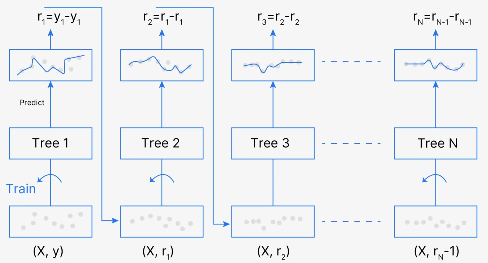
Description and Comments This figure provides a step-by-step illustration of the Gradient Boosting algorithm, where each tree is trained sequentially on the residuals (errors) of the previous tree, ultimately improving the model’s prediction accuracy. The process is depicted as follows:

• Initial Step: The first decision tree, denoted as Tree 1, is trained on the original data points $(X, y)$, where $X$ is the set of features and $y$ is the target variable. The model makes initial predictions $\hat{y}_1$, which have associated residuals $r_1 = y - \hat{y}_1$.

• Subsequent Trees (Residual Learning): For each subsequent tree, the algorithm fits the model to the residuals of the previous prediction. Tree 2 is trained on the residuals from Tree 1, denoted as $r_1$. Similarly, Tree 3 is trained on the residuals $r_2$ left by Tree 2, and this pattern continues through the $N$-th tree. Mathematically, the residuals $r_t$ for each tree $t$ are computed as:

  \[r_t = r_{t-1} - \hat{r}_{t-1},\]

  where $\hat{r}_{t-1}$ represents the prediction of the residuals by the $(t-1)$-th tree.

• Error Reduction (Gradient Direction): The goal of each tree in this sequence is to minimize the prediction error by reducing the residuals. Each tree makes adjustments in the gradient direction to correct the errors made by the previous trees, effectively "boosting" the accuracy of the overall ensemble model.

• Final Prediction (Ensemble): After $N$ trees have been trained, the final prediction is obtained by combining the predictions of all individual trees. The ensemble model aggregates these predictions, typically through a weighted sum, to make the final prediction, which is a refined and accurate approximation of the target variable $y$.

Classification

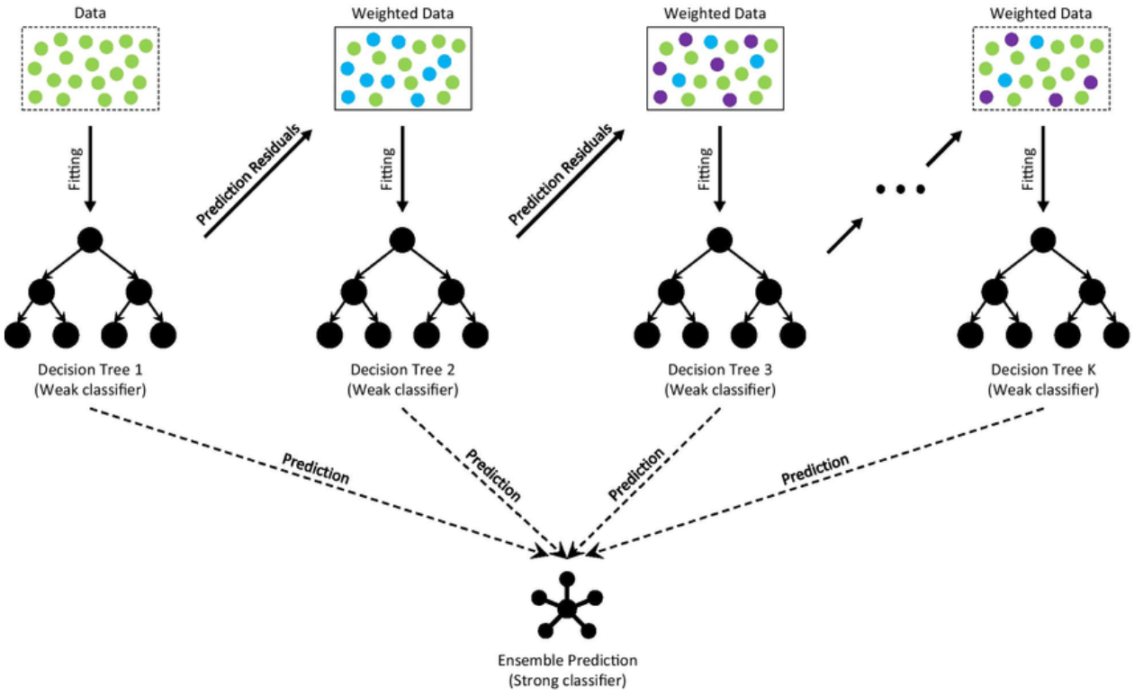
Description: The figure illustrates the process of building an ensemble model using Gradient Boosting with Decision Trees as weak classifiers. Each decision tree in the sequence is trained to fit the residuals (errors) of the previous trees, resulting in an incremental improvement in the model’s predictive accuracy.

• Data and Residuals: Initially, the model is trained on the full dataset. After each iteration, residuals (prediction errors) from the previous tree are calculated and used to weight the data for the subsequent tree.

• Weak Classifiers (Decision Trees): Each step in the boosting process adds a new weak classifier, typically a decision tree. The trees are denoted as Decision Tree 1, Decision Tree 2, ..., Decision Tree K. Each of these trees focuses on learning from the residuals of the previous ensemble.

• Weighted Data: With each iteration, the data points are reweighted based on the residuals from the previous tree. Points with higher residuals are given more weight so that subsequent trees focus more on these challenging instances.

• Ensemble Prediction: Once all the weak classifiers have been trained, their predictions are combined to form a strong classifier. The final prediction of the ensemble is a weighted sum of the predictions from each individual tree, resulting in a more accurate overall model.

This process continues iteratively, with each new tree aiming to correct the mistakes of the preceding trees, thereby reducing the overall prediction error and improving the model’s accuracy.

In classification tasks, common loss functions include:

• Logistic Loss (Log Loss): For binary classification, logistic loss measures performance by penalizing predictions that are probabilistically far from actual class labels. It is especially common in binary classification tasks.

  \[L(y, \hat{y}) = -\frac{1}{n} \sum_{i=1}^{n} \left[ y_i \log(\hat{y}_i) + (1 - y_i) \log(1 - \hat{y}_i) \right]\]

• Multinomial Deviance: Extending logistic loss to multiclass classification, multinomial deviance calculates error across multiple classes by penalizing probabilistic deviations.

  \[L(y, \hat{y}) = -\frac{1}{n} \sum_{i=1}^{n} \sum_{k=1}^{K} y_{i,k} \log(\hat{y}_{i,k})\]

  where $K$ is the number of classes, and $y_{i,k}$ is a binary indicator (0 or 1) indicating if class label $k$ is the correct classification for observation $i$.

Selecting the right loss function is key to maximizing model accuracy and effectiveness.

Additive Model

Gradient Boosting constructs an additive model by sequentially adding weak learners to minimize the loss function. Each learner is trained on the residuals of previous learners, improving the overall model iteratively.

Mathematically, the additive model can be described as:

\[F_{M}(x) = F_{0}(x) + \sum_{m=1}^{M} \eta h_{m}(x)\]

where:

• $F_{M}(x)$ is the final model after $M$ iterations.

• $F_{0}(x)$ is the initial model, typically a constant.

• $\eta$ is the learning rate, determining each weak learner’s contribution.

• $h_{m}(x)$ is the $m$-th weak learner.

The learning rate $\eta$ is crucial, balancing between the number of iterations and the contribution of each learner. A smaller $\eta$ often requires more iterations but can lead to better generalization by reducing overfitting.

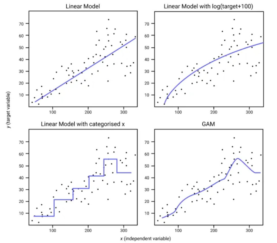
Description and Explanation: This figure compares the fits of different modeling approaches on a dataset with an independent variable $x$ and a target variable $y$. The models compared are as follows:

• Linear Model (Top Left): This model represents a simple linear regression fit. The straight line indicates that this model assumes a constant linear relationship between $x$ and $y$. While it captures the general upward trend, it fails to capture any non-linear patterns.

• Linear Model with Log Transformation of Target (Top Right): Here, a linear model is applied after a log transformation on the target variable, $\log(y + 100)$. The transformation allows the model to capture some of the non-linear pattern present in the data, resulting in a curve rather than a straight line. This approach helps when the relationship between $x$ and $y$ is non-linear, but it does not capture all details of the data distribution.

• Linear Model with Categorized $x$ (Bottom Left): In this approach, the continuous variable $x$ is categorized into discrete bins, and a linear model is fit on these categories. The result is a stepwise function, where each step represents the average response for that category. This approach can capture sudden changes and plateaus in the data but may miss finer details.

• Generalized Additive Model (GAM) (Bottom Right): The Generalized Additive Model (GAM) allows for a more flexible, non-linear relationship between $x$ and $y$ by fitting smooth functions to subsets of the data. The blue curve represents the model’s ability to adapt to the data’s underlying pattern more accurately than the previous approaches. GAM is useful for capturing complex, non-linear relationships without making strong assumptions about the form of the relationship.

Gradient Descent in Gradient Boosting

Gradient Boosting minimizes the loss function using gradient descent by iteratively adding weak learners that move in the direction of the negative gradient of the loss function. This process enables the model to adaptively refine predictions by focusing on residual errors.

The process can be summarized as follows:

1. Initialize the model with a constant prediction (such as the mean for regression or log-odds for classification).

2. Compute the negative gradient of the loss function with respect to the current model’s predictions to identify the residuals.

3. Fit a weak learner to the residuals, effectively addressing the errors from the prior model.

4. Update the model by scaling and adding the weak learner with a learning rate $\eta$:

   \[F_{m}(x) = F_{m-1}(x) + \eta h_{m}(x)\]

   where $F_{m}(x)$ is the updated model, $F_{m-1}(x)$ is the previous model, and $h_{m}(x)$ is the weak learner fitted to the residuals.

5. Repeat until convergence or a specified iteration count.

More details:

• Input: Training set ${(x_i, y_i)}_{i=1}^{n}$, a differentiable loss function $L(y, F(x))$, number of iterations $M$.

• Algorithm:

  1. Initialize the model with a constant value:

     \[F_0(x) = \arg \min_{\gamma} \sum_{i=1}^{n} L(y_i, \gamma).\]

  2. For $m = 1$ to $M$:

     1. Compute the pseudo-residuals:

        \[r_{im} = -\left[ \frac{\partial L(y_i, F(x_i))}{\partial F(x_i)} \right]_{F(x) = F_{m-1}(x)} \quad \text{for } i = 1, \ldots, n.\]

     2. Fit a weak learner $h_m(x)$ to the pseudo-residuals, using the training set ${(x_i, r_{im})}_{i=1}^{n}$.

     3. Compute the multiplier $\gamma_m$ by solving:

        \[\gamma_m = \arg \min_{\gamma} \sum_{i=1}^{n} L(y_i, F_{m-1}(x_i) + \gamma h_m(x_i)).\]

     4. Update the model: \(F_m(x) = F_{m-1}(x) + \gamma_m h_m(x).\)

  3. Output $F_M(x)$.

Regularization Techniques

Regularization in Gradient Boosting is essential to prevent overfitting, improving the generalizability of the model on unseen data. Various techniques include:

Shrinkage

Shrinkage, or learning rate regularization, modifies the update rule as:

\[F_m(x) = F_{m-1}(x) + \nu \cdot \gamma_m h_m(x), \quad 0 < \nu \leq 1\]

where $\nu$ is the learning rate. Small learning rates (e.g., $\nu < 0.1$) yield better generalization but require more iterations.

Stochastic Gradient Boosting

Stochastic Gradient Boosting is a variant of the standard Gradient Boosting algorithm introduced by Friedman. This modification is inspired by Breiman’s bootstrap aggregation, or "bagging," method. Specifically, it proposes that at each iteration, a base learner is fit on a random subsample of the training data without replacement.

Friedman observed a substantial improvement in Gradient Boosting’s accuracy with this modification.

The subsample size is represented by a constant fraction $f$ of the total training set size. When $f = 1$, the algorithm operates deterministically and is identical to the standard Gradient Boosting algorithm. However, smaller values of $f$ introduce randomness, which helps prevent overfitting and acts as a regularization technique. Additionally, the algorithm becomes faster, as each iteration uses a smaller dataset to fit the regression trees.

Typically, a subsample fraction $0.5 \leq f \leq 0.8$ provides good results for small to moderate-sized training sets. Setting $f = 0.5$ means that half of the training data is used to build each base learner.

Like bagging, subsampling in Stochastic Gradient Boosting allows for the definition of an out-of-bag error, which estimates the prediction improvement by evaluating the model on observations not used in the training of the base learner. This approach can replace an independent validation dataset, though out-of-bag estimates may underestimate actual performance improvements and the optimal number of iterations.

Number of Observations in Leaves

Gradient Tree Boosting implementations often include regularization by limiting the minimum number of observations in the terminal nodes (leaves) of trees. This constraint prevents splits that would result in nodes containing fewer than the specified minimum number of samples, thereby helping to reduce variance in predictions at leaves. By setting this limit, the model can achieve more stable and generalizable predictions.

Complexity Penalty

Another regularization technique in Gradient Boosting is to penalize model complexity. For Gradient Boosted Trees, model complexity can be defined in terms of the proportional number of leaves in the trees. A complexity penalty optimizes both the loss and the model’s structural complexity, which corresponds to a post-pruning approach where branches that fail to reduce the loss by a threshold are removed.

Additional regularization techniques, such as applying an $\ell_2$ penalty on the leaf values, can also be used to prevent overfitting. This penalization helps in achieving a balance between model flexibility and generalization ability.

Each method contributes to the model’s robustness, helping balance between fitting the data closely and generalizing well.

Feature Importance and Interpretability

Gradient Boosting can provide feature importance rankings, which help interpret which variables contribute most to the model’s predictions. This is typically done by aggregating the importance metrics of base learners, making it useful for understanding the relative impact of features in complex datasets. Despite these insights, Gradient Boosting’s ensemble nature can limit interpretability due to the complexity of the combined models.

Comparison between AdaBoost and Gradient Boosting

AdaBoost	Gradient Boosting
During each iteration in AdaBoost, the weights of incorrectly classified samples are increased, so that the next weak learner focuses more on these samples.	Gradient Boosting updates the weights by computing the negative gradient of the loss function with respect to the predicted output.
AdaBoost uses simple decision trees with one split known as the decision stumps of weak learners.	Gradient Boosting can use a wide range of base learners, such as decision trees and linear models.
AdaBoost is more susceptible to noise and outliers in the data, as it assigns high weights to misclassified samples.	Gradient Boosting is generally more robust, as it updates the weights based on the gradients, which are less sensitive to outliers.

Variants of Gradient Boosting

Over time, several variants of Gradient Boosting have emerged, optimizing the standard algorithm for specific applications and computational efficiency:

LightGBM

LightGBM (Light Gradient Boosting Machine) is a high-performance gradient boosting framework developed by Microsoft, optimized for speed and efficiency on large-scale datasets. Unlike traditional gradient boosting algorithms, LightGBM introduces several key innovations:

• Leaf-Wise Tree Growth: LightGBM grows trees leaf-wise rather than level-wise, splitting the leaf with the largest loss reduction, often resulting in higher accuracy and deeper trees.

• Histogram-Based Algorithm: Continuous feature values are bucketed into discrete bins, significantly reducing memory usage and computation time.

• Gradient-Based One-Side Sampling (GOSS): LightGBM retains only the data points with large gradients, focusing on the most informative samples to speed up training without sacrificing performance.

• Exclusive Feature Bundling (EFB): LightGBM combines sparse features into a single feature, reducing the number of features and improving efficiency.

LightGBM is known for its speed and low memory usage, making it suitable for large, high-dimensional datasets. Its ability to handle sparse data, support parallel and distributed learning, and leverage modern hardware like GPUs has made it popular in applications such as financial modeling, ranking problems, and real-time prediction systems.

CatBoost

CatBoost is an open-source gradient boosting library developed by Yandex, initially released in July 2017. Unlike traditional gradient boosting frameworks, CatBoost is specifically designed to handle categorical features efficiently using a permutation-driven approach, which helps mitigate overfitting issues. Key features of CatBoost include:

• Native Handling of Categorical Features: CatBoost natively supports categorical features, making it a powerful tool for datasets with non-numeric data.

• Ordered Boosting: This technique helps to reduce overfitting by using ordered statistics to process categorical data.

• Oblivious Trees: CatBoost utilizes symmetric, or oblivious, trees for faster execution.

• Fast GPU Training: Optimized for GPU training, CatBoost provides efficient training on large datasets.

• Cross-Platform and Language Support: CatBoost supports Python, R, C++, Java, and models can be exported to other formats such as ONNX and Core ML.

CatBoost has gained recognition and is widely used in the machine learning community, ranking among the top frameworks in Kaggle’s surveys and receiving awards like InfoWorld’s "Best Machine Learning Tools" in 2017.

XGBoost

XGBoost (eXtreme Gradient Boosting) is an open-source gradient boosting library initially released in March 2014. Developed by Tianqi Chen and maintained by the Distributed (Deep) Machine Learning Community (DMLC), XGBoost is known for its efficiency, scalability, and competitive performance in machine learning competitions. XGBoost supports a wide range of languages, including C++, Python, R, Java, and Scala, and can operate on Linux, macOS, and Windows. It is compatible with single-machine setups as well as distributed frameworks like Apache Hadoop, Apache Spark, Apache Flink, and Dask.

Some unique features of XGBoost include:

• Regularization: XGBoost applies clever penalization to tree structures to prevent overfitting.

• Newton Boosting: A second-order gradient boosting technique for more accurate optimization.

• Sparsity-Aware Algorithms: Efficient handling of sparse data with parallel tree boosting.

• Leaf Node Shrinking: Proportionally shrinks leaf nodes to improve model generalization.

• Integration with Distributed Systems: Supports scalable, distributed training across various data processing frameworks.

XGBoost gained popularity due to its high accuracy and has been the preferred algorithm for many winning solutions in ML competitions, despite the reduced interpretability compared to simpler models like single decision trees.

Applications of Gradient Boosting

Gradient Boosting has widespread applications in both industry and academia. Some of its common use cases include:

• Financial Modeling: Used in credit scoring, risk assessment, and fraud detection, where accuracy is paramount.

• Healthcare: Applied in predictive diagnostics, personalized treatment recommendations, and analyzing complex medical datasets.

• E-commerce: Employed in recommendation systems, demand forecasting, and pricing optimization to enhance customer experience.

• Natural Language Processing (NLP): Utilized in text classification, sentiment analysis, and language translation.

• Ranking and Search Engines: Many search engines, such as Yahoo and Yandex, utilize Gradient Boosting in their ranking algorithms for more accurate search results.

• Scientific Research: High Energy Physics experiments, like those at the Large Hadron Collider, use Gradient Boosting to analyze particle collisions and confirm theoretical predictions.

Gradient Boosting’s flexibility and power make it a preferred method for various predictive modeling applications.

Disadvantages of Gradient Boosting

While Gradient Boosting can significantly improve the accuracy of weak learners, it also has notable drawbacks:

• Computational Intensity: Gradient Boosting can be slow to train, especially with a large number of iterations or complex base learners.

• Overfitting Risk: Without careful regularization, it can overfit the training data, especially if the model complexity is high.

• Interpretability: As an ensemble of weak learners, Gradient Boosting sacrifices interpretability. Following the decision path across hundreds or thousands of trees is difficult.

Some advanced techniques, such as model compression or surrogate models, have been developed to approximate the decision function of Gradient Boosting with simpler, interpretable models.